Tutorial 2: Medical CT, From AI Segmentation to Simulation

This tutorial follows a contrast-enhanced abdominal and pelvic CT scan through a complete anatomical workflow: reviewing an automated multi-label segmentation, editing and extracting labels, adding structures the model missed with semi-automatic tools, converting masks into surfaces, turning surfaces into simulation-ready tetrahedral meshes, and measuring and reporting the result.

Estimated time: 75 minutes

Level: Intermediate to advanced

Dataset: samples\tutorial-data\tutorial-2

Medical Disclaimer

Volvicon is not a regulated medical device. It has not been cleared by the FDA, CE marked, or approved by any other regulatory body for clinical diagnosis, treatment planning, or medical decision making. Segmentation and measurement results in this tutorial are for training only and must be reviewed and validated by qualified professionals before any clinical use.

---

What You Will Learn

1. Read a multi-label segmentation produced by an AI model and judge its quality slice by slice.
2. Rename, recolour, combine, remove, and extract labels with the Multi-label Mask Editor.
3. Segment a structure the model missed using Dynamic Region Grow, and extend it with the Merge mode.
4. Refine a mask by hand with brushes, morphology, and region filters.
5. Generate clean surfaces from masks and repair them.
6. Build tetrahedral volume meshes and check their element quality.
7. Measure anatomy, compare segmentations, and export a report.
8. Optionally run your own AI model on the volume.

---

The Dataset

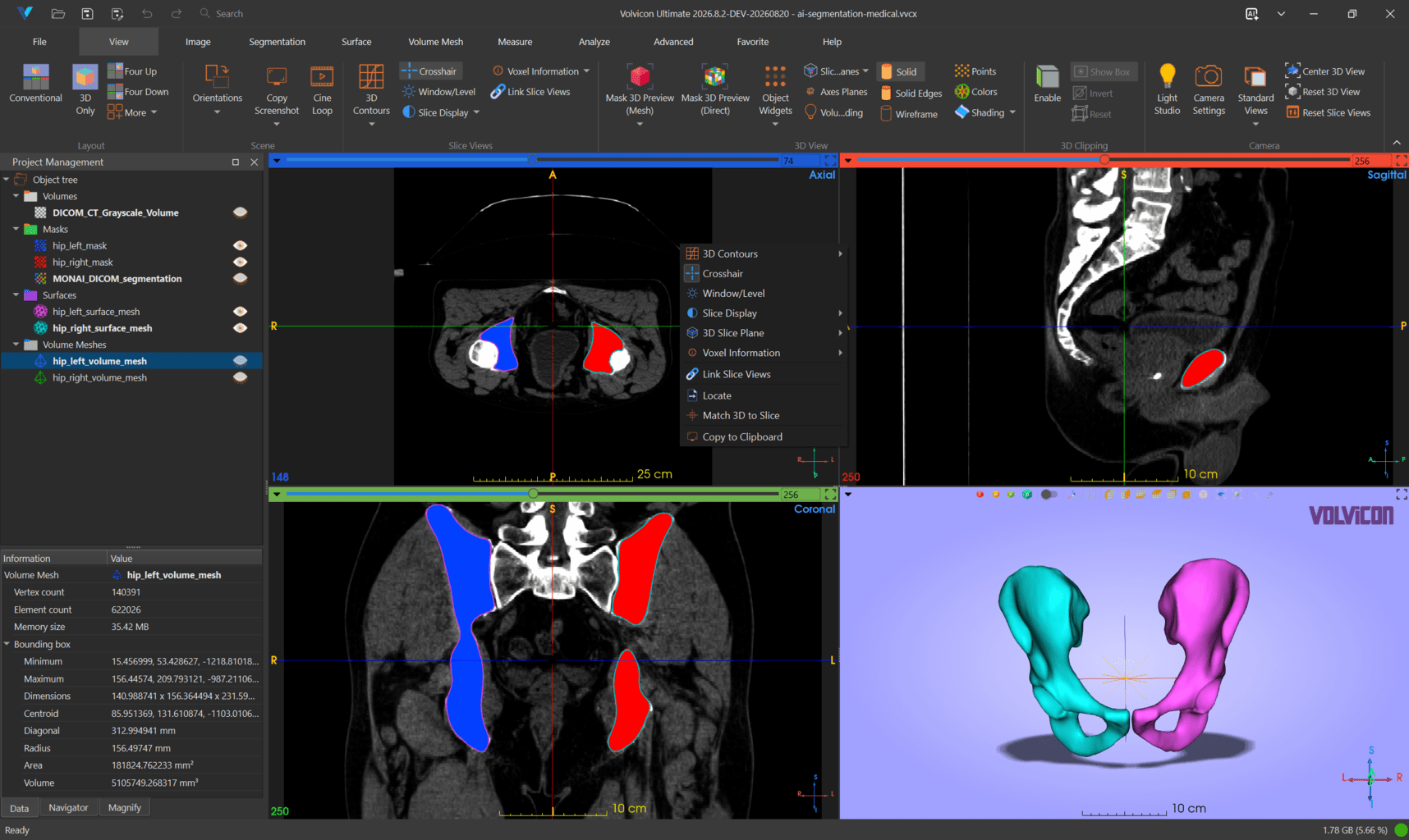
Scene tree objects

Type	Name	Description
Volume	DICOM_CT_Grayscale_Volume	The imported CT series
Mask	MONAI_DICOM_segmentation	Multi-label AI segmentation with 29 labelled structures
Mask	hip_left_mask	Binary mask of the left hip bone, extracted from the multi-label mask
Mask	hip_right_mask	Binary mask of the right hip bone
Surface	hip_left_surface_mesh	Triangle mesh generated from hip_left_mask
Surface	hip_right_surface_mesh	Triangle mesh generated from hip_right_mask
Volume Mesh	hip_left_volume_mesh	Tetrahedral mesh generated from the left hip surface
Volume Mesh	hip_right_volume_mesh	Tetrahedral mesh generated from the right hip surface

Volume properties

Property	Value
Voxel grid	512 x 512 x 149
Voxel spacing	0.9766 x 0.9766 x 2.0 mm
Physical size	about 500 x 500 x 298 mm
Voxel type	Signed 16-bit
Gray value range	-1000 to 2976 HU
Source	DICOM series

Because this volume was imported from DICOM, its gray values are calibrated Hounsfield units. The window and level presets and the threshold presets in Volvicon are built for exactly this scale, which is the main practical difference from the industrial dataset in Tutorial 1.

The 29 segmented structures

MONAI_DICOM_segmentation stores every structure in one mask, each with its own integer label value and annotation.

Value	Structure	Value	Structure	Value	Structure
6	stomach	55	small_bowel	95	gluteus_maximus_right
7	aorta	56	duodenum	96	gluteus_medius_left
8	inferior_vena_cava	57	colon	97	gluteus_medius_right
18	vertebrae_L5	88	femur_left	98	gluteus_minimus_left
19	vertebrae_L4	89	femur_right	99	gluteus_minimus_right
20	vertebrae_L3	90	hip_left	100	autochthon_left
51	iliac_artery_left	91	hip_right	101	autochthon_right
52	iliac_artery_right	92	sacrum	102	iliopsoas_left
53	iliac_vena_left	94	gluteus_maximus_left	103	iliopsoas_right
54	iliac_vena_right			104	urinary_bladder

The label values are not consecutive because they come from the model's own label map. Volvicon preserves them, which keeps the segmentation interoperable with the model that produced it.

---

Part 1: Open the Project and Set Up for Anatomy

Step 1.1: Open the project

1. Go to File ▸ Open ▸ Computer ▸ Browse.
2. Select ai-segmentation-medical.vvcx from your copy of tutorial-2 and click Open.

Step 1.2: Choose a medical orientation

Go to View ▸ Scene ▸ Orientations and select Medical 1 (radiologist convention) or Medical 2 (neurologist convention). The orientation preset changes axis labels, view directions, and slice names throughout the interface. It does not change the voxel data.

With a medical preset the slice views are named Plane 1 (YZ), Plane 2 (XZ), and Plane 3 (XY), and the direction labels read Left, Right, Anterior, Posterior, Superior, and Inferior.

Step 1.3: Set a diagnostic window

1. Open View ▸ Slice Views ▸ Window/Level. If a gray value interval mode is active, answer Yes to switch the slice display back to Standard.
2. In the Presets list, select CT-Bone (level 400, window 1000). The skeleton becomes sharply defined.
3. Switch to CT-Abdomen (level 40, window 350) and note how the soft tissue structures separate instead.
4. Try a colour lookup table from the Lookup table list to distinguish ranges that look alike in grayscale.

Each preset shows a thumbnail of the middle axial slice rendered with that preset, so you can compare the list at a glance.

Step 1.4: Turn on the navigation aids

1. Enable Crosshair from the slice view context menu.
2. Set Voxel Information to Both.
3. Hover over the pelvis. The readout shows the world position, the voxel index, and the HU value. Over a visible mask it also shows the mask name, and for a multi-label mask the label number with its annotation, so you can identify a structure just by pointing at it.

---

Part 2: Reviewing the AI Segmentation

Step 2.1: See the segmentation in 2D and 3D

1. Make MONAI_DICOM_segmentation the active mask and turn on its visibility.
2. Scroll through the axial slices. Every structure is drawn in its own colour.
3. Turn on View ▸ 3D View ▸ Mask 3D Preview (Direct). The mask is rendered directly on the GPU with no mesh generation, which is the fastest way to look at a 29-label segmentation.
4. Now click the green O button on the 3D view toolbar to generate a Mask 3D Preview (Mesh) at Optimal quality instead. Direct mode is switched off automatically, because the two modes are mutually exclusive.

Preview mode	Strengths
Direct	Instant, shows edits immediately, no mesh step, good during active editing
Mesh	Real geometry, required by surface based tools and mask analyses, accurate at Optimal quality

Multi-label surface extraction

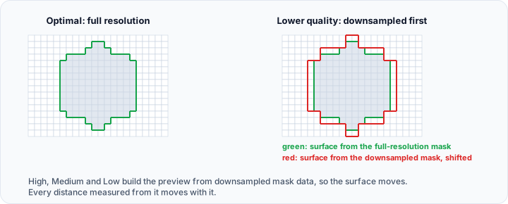
How each label's preview surface is built is configured in File ▸ Preferences ▸ 3D View ▸ Mask 3D preview settings ▸ Multilabel mask. Accurate surface detection is enabled by default and builds every label independently as a smooth, closed surface, which is the right choice for measurement and per-label export. Turning it off exposes three faster alternatives for visualisation-only previews. See 3D View.

Step 2.2: Open the Multi-label Mask Editor

With MONAI_DICOM_segmentation active, go to Segmentation ▸ Operations ▸ Multi-label Mask ▸ Multi-Label Mask Editor.

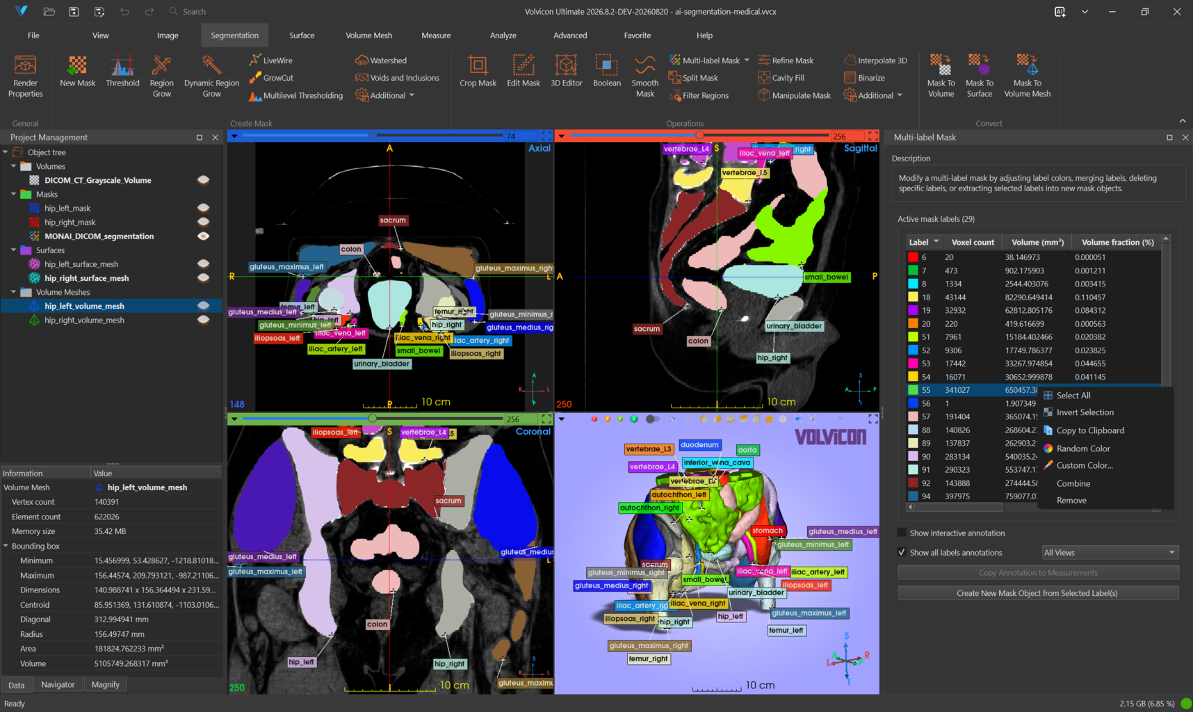
The Active mask labels table lists all 29 labels with their colour swatch, their statistics, and their annotation, and the group title shows the label count in brackets.

Step 2.3: Judge and clean the segmentation

Work down the table and check each structure against the slice views. AI models are reliable on large, high-contrast organs and less reliable on thin, low-contrast, or partially imaged ones.

Use the right-click menu on the table to act on the selection:

Command	Effect
Select All / Invert Selection	Change which rows are selected
Copy	Copy the selected rows to the clipboard
Random Color	Assign fresh random colours to the selected labels
Custom Color...	Pick one colour for the selection
Combine	Merge the selected labels into a single label
Remove	Delete the selected labels from the mask

Try both structural commands:

1. Select gluteus_maximus_left, gluteus_medius_left, and gluteus_minimus_left, right-click, and choose Combine. The three labels become one gluteal group.
2. Press Ctrl+Z to undo.
3. Select small_bowel, duodenum, and colon, right-click, and choose Remove to drop the bowel from the segmentation.
4. Press Ctrl+Z to undo.

Step 2.4: Extract the hip bones

This is how a standalone binary mask such as hip_left_mask is obtained from a multi-label segmentation.

1. In the table, select the row for label 90 (hip_left).
2. Click Create New Mask Object from Selected Label(s).
3. A new mask object appears in the scene tree, containing only that structure. The multi-label mask is unchanged.
4. Rename it by double-clicking its name in the scene tree, or by right-clicking and choosing Rename.
5. Repeat for label 91 (hip_right).

Compare your results with the shipped hip_left_mask and hip_right_mask.

Step 2.5: Annotate for review and presentation

• Enable Show interactive annotation, then click a table row or pick a structure in the 3D view. A label annotation appears at that structure's first voxel in every view.
• Enable Show all labels annotations and choose All Views from the adjacent list to label every structure at once. Annotations are repositioned automatically so they do not overlap.
• Click Copy Annotation to Measurements to move the active annotation into the Measurements tool, where it becomes part of a measurement report.

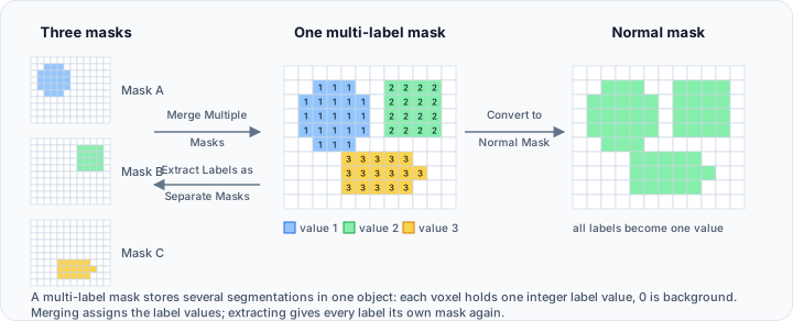
The other entries in the Multi-label Mask menu are Merge Multiple Masks, which builds one multi-label mask from several binary masks, Extract Labels as Separate Masks, which splits every label into its own object in a single operation, and Convert to Normal Mask(s), which discards the label information. All four are pages of the same panel, so you can also switch between them in the Operations list at the top of the tool.

Step 2.6: Quantify every structure

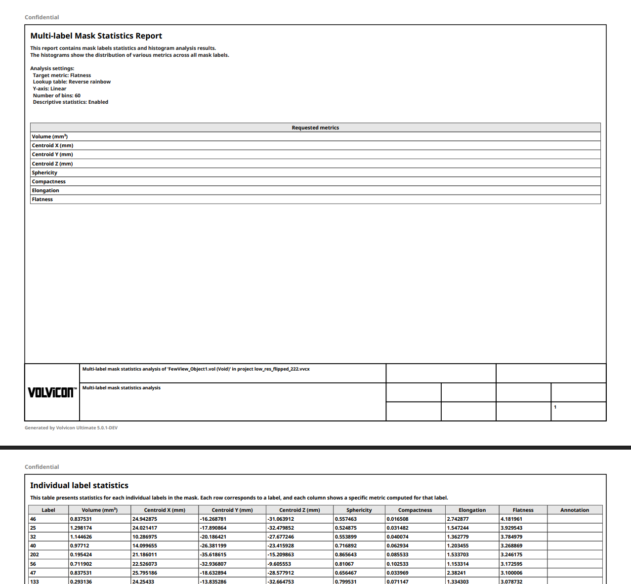
1. Keep MONAI_DICOM_segmentation active.
2. Go to Measure ▸ Statistics ▸ Mask Statistics ▸ Per-Label Mask Statistics.
3. Click the ... button next to Select statistics: and check the measurements you need, for example Volume (mm³), Volume fraction (%), Surface area (mm²), Sphericity, and Mean gray value.
4. Choose a Target metric: and a Lookup table:. The labels are recoloured from the lookup table by the selected metric, so relative organ volumes become visible at a glance.
5. Read the three tables: Individual label statistics, Overall descriptive statistics, and Whole mask statistics.
6. Click Export... for a CSV file or a PDF report.

The 3D recolouring needs a mesh preview

Recolouring the 3D preview and showing the colour scale requires a valid mask preview surface. If the 3D view does not change, generate the preview with the green O button on the 3D view toolbar and run the statistics again.

---

Part 3: Semi-Automatic Segmentation with Dynamic Region Grow

An automatic model segments what it was trained on. Anything else you add yourself. Dynamic Region Grow is the fastest way to capture a connected structure with reasonably uniform intensity, such as a contrast-filled vessel or a bone that the model left out.

Step 3.1: Configure the tool

1. Make DICOM_CT_Grayscale_Volume the active volume.

2. Go to Segmentation ▸ Create Mask ▸ Dynamic Region Grow.

3. Set Region growing method to Connectivity. This grows from a seed point using the statistical properties of its neighbourhood, rather than a fixed intensity range.

4. Set the parameters:

   Parameter	Value	Meaning
   Multiplier	2	Width of the confidence interval for intensity similarity. Larger values grow further.
   Number of iterations	2	How often the filter re-estimates the statistics and grows again.
   Initial neighborhood radius (pixels)	2	Size of the neighbourhood sampled around the seed.

5. In Options, leave Multiple layer checked so the region grows in 3D across all slices. Unchecked, it stays on the current slice.

6. In Result, leave the target mask on <New mask object> and the mode on Replace.

Step 3.2: Place the first seed

Left-click on the structure of interest in any 2D or 3D view. The region grows immediately from that point, and the result is written to a new mask object.

Inspect the result in all three slice views before you continue. If the region leaked into a neighbouring structure, undo with Ctrl+Z, lower the Multiplier, and try again. If it stopped too early, raise the Multiplier or the Number of iterations.

Seeding well

Place the seed in a representative, homogeneous part of the structure, away from partial-volume boundaries and away from metal or beam-hardening artefacts. The statistics sampled at the seed decide everything that follows.

Step 3.3: Name the result

A mask called Mask 1 is worthless three days later. Rename it now:

• Double-click the name in the scene tree and type a new one, or
• Right-click the mask and choose Rename.

Duplicate names are adjusted automatically so that every object stays uniquely identifiable.

Step 3.4: Add the regions that were missed

A single seed rarely captures a branched or partially disconnected structure. Extend the same mask instead of creating a second one:

1. Back in the Dynamic Region Grow panel, select your newly renamed mask in the Result target mask list.
2. Select the Merge radio button. Replace would overwrite what you already have; Merge adds to it.
3. Click on a region that is still missing in a slice view. The newly grown region is merged into the existing mask.
4. Repeat for every missing part, checking the result after each click.

This click, review, click loop is the core of semi-automatic segmentation. Because each click is a separate operation, Ctrl+Z removes only the last addition.

Step 3.5: Refine by hand

Open Segmentation ▸ Operations ▸ Edit Mask for voxel-level control:

Tool	Use
Brush	Paint or erase freehand. Left-click and drag.
Rectangle, Circle, Lasso	Left-click and drag, release to apply.
Polygon	Left-click to add vertices, middle-click to close and apply.
LiveWire	Semi-automatic edge tracing along image boundaries.
Level Tracing	Intensity-based boundary tracing, left-click and drag.

Shortcuts while the tool is open:

Shortcut	Action
Shift (hold)	Temporarily switch from Draw to Erase
+ / -	Increase or decrease the brush size
Ctrl+Shift+B	Toggle the brush shape between Circle and Rectangle

Enable Multiple Layer to apply an ROI through all slices, or leave it off to edit the current slice only. Threshold mode restricts drawing to voxels inside a gray value range, which lets you paint roughly over bone without picking up the surrounding soft tissue.

Step 3.6: Clean up with the mask operations

Tool	What it fixes
Smooth Mask	Jagged borders, using a discrete gaussian, recursive gaussian, mean, or median filter
Cavity Fill	Internal cavities left inside the structure
Filter Regions	Small disconnected specks, or oversized regions
Refine Mask	Artifacts and small holes in one pass
Manipulate Mask	Hollow, grow, or shrink the boundary
Interpolate 3D	Fill the gaps when you segmented only every few slices
Boolean	Union, intersection, or difference against another mask
Split Mask	Separate disconnected regions into individual mask objects
Binarize	Convert partial-volume values into strictly on or off voxels

Segment every second slice

For a structure with a smooth cross-section, segment every third or fourth slice with LiveWire or the brush, then run Interpolate 3D. It is often faster than segmenting every slice and gives a smoother result.

---

Part 4: From Masks to Surfaces

Step 4.1: Generate a surface

1. Make hip_left_mask the active mask.

2. Go to Segmentation ▸ Convert ▸ Mask To Surface.

3. Set Target object(s) to Active mask object.

4. Set Quality to Optimal for a full-resolution mesh, or to Custom to control each option yourself:

   Option	Effect
   Resolution reduction	Downsamples in XY and Z before extraction. Use it on very large masks.
   Filter shells	Keeps only the given number of largest shells by area.
   Smoothing	Iterations, smooth factor, and feature angle. Lower smooth factors smooth more; smaller feature angles preserve sharp edges.
   Triangle reduction	Percentage of triangles removed after extraction.

5. Click Apply. The new surface appears in the scene tree.

Compare your surface with the shipped hip_left_surface_mesh.

Smooth the mask, not only the surface

Applying Smooth Mask before conversion produces a cleaner surface than heavy smoothing afterwards, because smoothing the mesh moves vertices away from the segmented boundary.

Step 4.2: Repair before you go further

Run Surface ▸ Edit ▸ Diagnostics and Fixes on the new surface:

1. On the Quick Fix tab, click Update to run all diagnostics.
2. Review which fix options are enabled, since several of them can remove geometry.
3. Click Fix, then Update again.
4. Confirm the Comments section reports that the surface is closed and manifold.
5. Use the Holes tab to close any remaining open boundaries, and the Normals tab to correct inverted triangles.

This step is mandatory before Boolean operations, volume meshing, 3D printing, or any thickness measurement. A surface extracted from a segmentation is rarely defect-free.

Step 4.3: Control triangle count and quality

Tool	Use
Smooth	Reduce residual voxel stepping
Reduce	Decimate the triangle count while preserving shape
Remesh	Rebuild triangles with uniform size and better shape quality
Subdivide	Increase resolution where you need finer detail
Filter Shells	Drop small artefact components

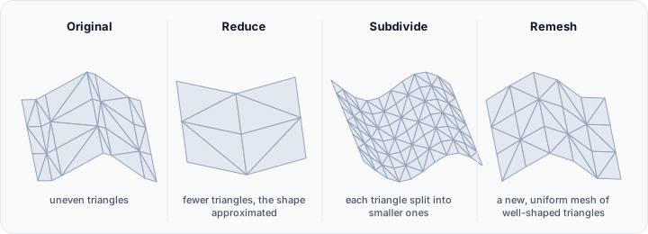
Check the outcome with Measure ▸ Statistics ▸ Surface Statistics and Measure ▸ Analysis ▸ Mesh Quality Analyzer ▸ Surface Quality. For a mesh that will be tetrahedralised, aim for triangle angles between 30 and 90 degrees and aspect ratios close to 1.

---

Part 5: Simulation-Ready Volume Meshes

Step 5.1: Inspect the shipped meshes

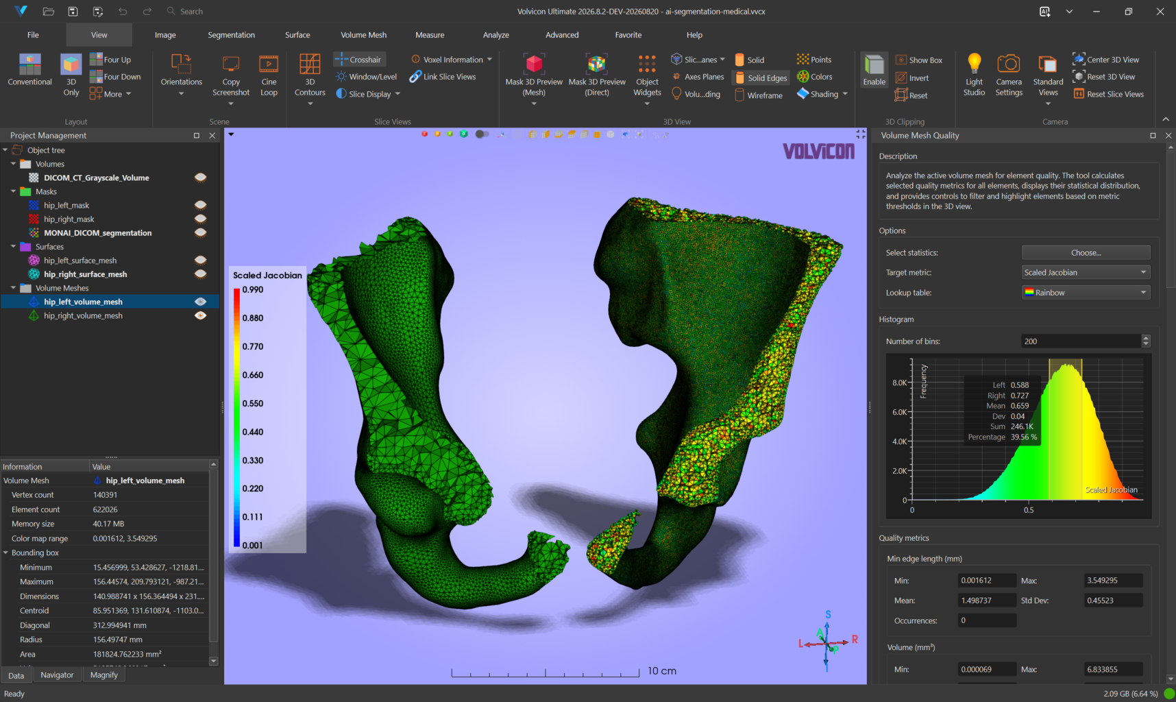
Make hip_left_volume_mesh visible and active, hide the volume and the masks, and press E in the 3D view for Solid Edges. The Properties tab reports element and vertex counts, memory, and bounding box measurements.

Step 5.2: Create your own

1. Make your repaired hip surface active.

2. Go to Surface ▸ Convert ▸ Surface To Volume Mesh.

3. Choose the algorithm and the element type:

   Element type	Choose it for
   Tetra 4-node (linear)	Preliminary analysis, large models, lower computational cost
   Quadratic 10-node	Stress analysis, curved boundaries, contact and other nonlinear problems

4. When you convert the left and right hip together, decide whether to maintain conformity so that shared interfaces receive matching node positions.
5. Apply.

Watertight input required

Tetrahedralisation needs a closed, manifold surface with consistent outward normals and no self-intersections. If it fails, return to Diagnostics and Fixes rather than changing meshing parameters.

Step 5.3: Check element quality

Open Measure ▸ Analysis ▸ Mesh Quality Analyzer ▸ Volume Mesh Quality. Select the metrics to compute, pick a Target metric, and read the distribution. Drag across the chart to mark a range of values: the marked range reports its borders, mean, standard deviation, total, and share of the mesh, which quantifies a group of poor elements before you decide what to do about them.

Step 5.4: Configure and export for a solver

1. Go to Volume Mesh ▸ FEM ▸ Configure FEM Model to define material properties, boundary conditions, and element sets.
2. Go to Volume Mesh ▸ FEM ▸ Export FEM Mesh and choose your solver format.
3. To bring a mesh back from a solver, use File ▸ Import ▸ Volume Mesh Models, or drag the solver file onto the 3D view. Where the file provides them, materials, node and element sets, surfaces, and parts are imported with the mesh.
4. Volume Mesh ▸ Convert ▸ Volume Mesh To Surface extracts the boundary surface again, which is a quick way to verify what the solver actually receives.

For a deeper treatment, see Volume Mesh for Simulation.

---

Part 6: Measuring Anatomy

Step 6.1: Linear and angular measurements

1. Go to Measure ▸ Measurement tools ▸ Measurements.
2. Select Distance and click the green + button to enter placement mode.
3. Click two points across the femoral head in a slice view, or on the surface in the 3D view. The distance in millimetres appears in the table and as an annotation.
4. Grab either handle and drag it. On a surface in the 3D view the handle follows the geometry and the value updates live.

5. Select Angle and place three points, with the vertex in the middle, to measure an anatomical angle. 6. Select Diameter and place three points on a circular cross-section such as the aorta. 7. Right-click a row and choose Locate to bring every slice view to that measurement. 8. Use Save in the toolbar to export the measurements as an INI file. Volvicon stores a SHA-256 integrity hash with the file and verifies it on import, warning you if the file was modified outside the application.

Step 6.2: Reference geometry with primitives

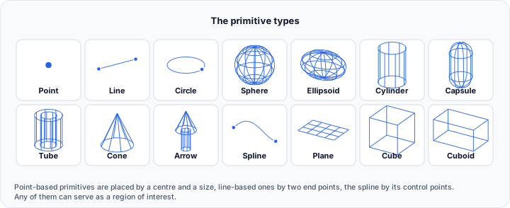
Go to Measure ▸ Primitive tools ▸ Primitives, select Sphere, click the + button, then click to set the centre and drag to define the radius. Fit it to the femoral head and read its parameters.

Primitive Fitting fits primitives to surface geometry automatically, and Measurement between Primitives measures distances and angles between them, for example between a fitted sphere centre and a fitted plane.

Step 6.3: Compare two segmentations

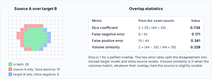
Measure ▸ Statistics ▸ Compare Masks calculates overlap statistics between two masks. Compare your hand-corrected mask against the original AI label to quantify how much you changed, which is the standard way to document a manual correction.

Step 6.4: Produce the report

Click Export... in any statistics, measurement, or analysis tool and choose the PDF report. The PDF Report dialog generates a formatted document containing the analysis settings, the tables, the charts, the measurements, snapshots of the views, and an interactive 3D scene. See PDF Report Generation for the full set of options.

---

Part 7 (Optional): Run Your Own AI Segmentation

The segmentation in this project came from a MONAI whole-body CT model. You can reproduce it on the same volume.

Research use only

The AI segmentation functionality is intended for research purposes and is not approved for clinical or diagnostic use. Results must always be reviewed and validated by qualified professionals.

Step 7.1: Install a framework

Run Volvicon as administrator, open Advanced ▸ Artificial Intelligence ▸ AI Segmentation, select the framework, and click its Install button. The download and configuration are handled for you, and Volvicon must be restarted afterwards. See AI Segmentation for the alternative manual installation and for troubleshooting.

Volvicon integrates four frameworks:

Framework	Scope
TotalSegmentator	Whole-body CT segmentation covering 117 anatomical structures
nnU-Net	Self-configuring framework for medical image segmentation
MONAI	Pre-trained model bundles, including whole-body CT segmentation
Cellpose-SAM	Instance segmentation for cells, nuclei, and densely packed objects

Step 7.2: Run a MONAI bundle

1. Obtain a MONAI bundle with the expected configs, models, scripts, and docs structure. Single-channel 3D segmentation bundles such as wholeBody_ct_segmentation are supported; 2D models, multi-channel models, and detection models are not.
2. In the AI Segmentation panel, select MONAI and set the Bundle Directory, the Config File (normally configs/inference.json), and the Model File (normally models/model.pt).
3. Choose the Device (CPU or GPU) and confirm the ROI Size, which is detected from the bundle.
4. Adjust the advanced options if memory is tight: Sliding Window Batch Size, Overlap, and the blending Mode.
5. Run the segmentation and monitor the progress and debug output. The result appears as a multi-label mask in the scene tree.

Orientation

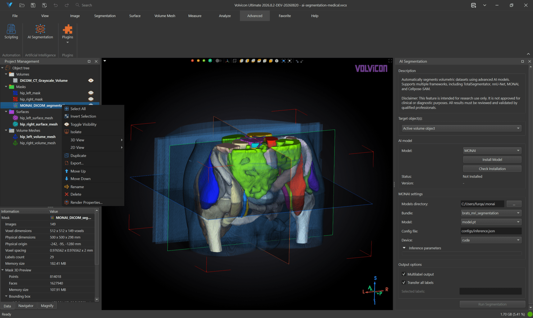
MONAI and Cellpose-SAM use the volume's current orientation. TotalSegmentator and nnU-Net require RAS orientation, which Volvicon supplies through the Make image orientation compatible option in the Output options panel. Leave it enabled for standard DICOM-imported volumes, and disable it only if you converted the volume to RAS yourself beforehand.

Step 7.3: Review what the model produced

Whatever framework you use, the output is a multi-label mask, and the review workflow is the one you already know from Part 2: open the Multi-label Mask Editor, check each structure against the slice views, correct what is wrong, and extract what you need.

---

What You Have Built

• A reviewed and corrected 29-structure segmentation of an abdominal and pelvic CT.
• Binary masks extracted from individual labels.
• An additional structure segmented semi-automatically and refined by hand.
• Repaired triangle surfaces suitable for measurement and export.
• Tetrahedral volume meshes with verified element quality.
• Anatomical measurements, comparison statistics, and a report.

---

Next Steps

Direction	Where to go
Import your own DICOM data	Tutorial 3: DICOM Import and Semi-Automatic Segmentation
Industrial inspection workflows	Tutorial 1: Industrial CT Inspection
More on AI segmentation	AI-Powered Segmentation
More on simulation meshes	Volume Mesh for Simulation
Reference for any tool used here	GUI Reference