Tutorial 1: Industrial CT Inspection

This tutorial takes a reconstructed industrial CT scan of a manufactured part from first look to finished inspection report and presentation video. You will work through nine ribbon tabs on one dataset, and by the end you will have measured the part, found and quantified its internal defects, repaired and analysed its surface, automated the whole thickness workflow in Python, and rendered an animation of the result.

Estimated time: 90 minutes

Level: Intermediate to advanced

Dataset: samples\tutorial-data\tutorial-1

Industrial Use Disclaimer

The measurements and analyses produced in this tutorial are for training purposes. Inspection results used for acceptance decisions must be validated against the applicable standard by a qualified inspector, with documented parameters and a calibrated acquisition.

---

What You Will Learn

1. Read and shape a 16-bit CT volume with the interactive gray value histogram.
2. Navigate slices, set contrast, and cut the 3D scene open at a slice plane.
3. Create, edit, and convert masks, including a multi-label defect mask.
4. Diagnose and repair a triangle mesh before any measurement is taken.
5. Quantify gray values, mask labels, surfaces, and volume meshes.
6. Run wall thickness and void/inclusion analyses and read their results.
7. Reproduce an entire analysis workflow from a Python script.
8. Compose and record a multi-track animation of the finished scene.

---

The Dataset

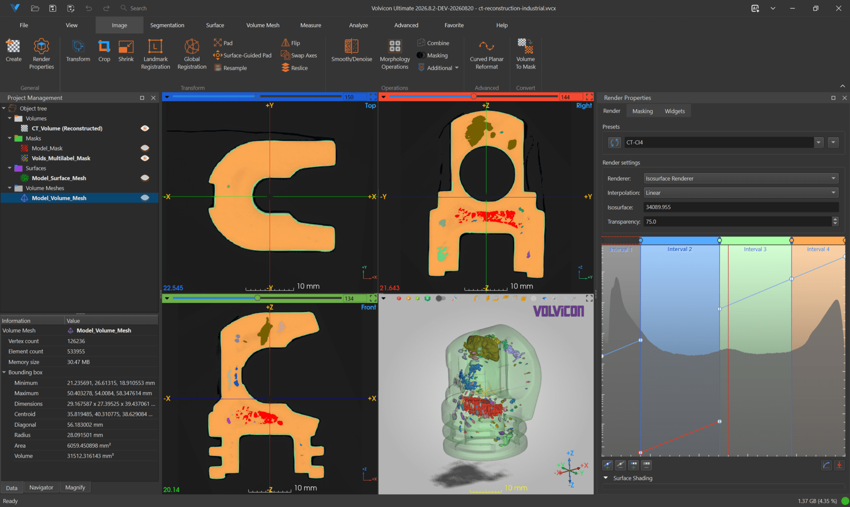
Open the project as described in Part 1, then compare what you see with the tables below.

Scene tree objects

Type	Name	Description
Volume	CT_Volume (Reconstructed)	The reconstructed CT scan of the part
Mask	Model_Mask	Binary mask of the solid material
Mask	Voids_Multilabel_Mask	Multi-label mask, one label per detected internal defect
Surface	Model_Surface_Mesh	Triangle mesh of the outer part geometry
Volume Mesh	Model_Volume_Mesh	Tetrahedral mesh generated from the part

Volume properties

Property	Value
Voxel grid	289 x 268 x 301
Voxel spacing	0.1503 mm, isotropic
Physical size	about 43.4 x 40.3 x 45.2 mm
Voxel type	Unsigned 16-bit
Gray value range	0 to 65535

Gray values, not Hounsfield units

This is an industrial CT reconstruction, so the gray values are relative attenuation values on a 16-bit scale, not calibrated Hounsfield units. Thresholds are therefore chosen from the histogram of this specific dataset, and the values in this tutorial do not transfer to other scans.

---

Part 1: Open the Project and Tour the Workspace

Step 1.1: Open the project

1. Go to File ▸ Open.
2. Select Computer in the left panel.
3. Click Browse, navigate to your copy of tutorial-1, and select ct-reconstruction-industrial.vvcx.
4. Click Open.

Volvicon verifies the integrity of the project while it loads, restores every object with its saved colours, opacity, and camera position, and shows the scene.

Integrity warnings

If a warning about the integrity manifest appears, the file was modified after it was saved. For the shipped sample this should not happen. Re-copy the file from the installation folder if it does.

Step 1.2: Read the scene tree

The Project Management dock on the left contains the scene tree with four fixed sections: Volumes, Masks, Surfaces, and Volume Meshes. Confirm that all five objects listed above are present.

Try the following:

• Click CT_Volume (Reconstructed). It becomes active and its name is shown in bold.
• Click the visibility icon next to Model_Surface_Mesh to show it, and again to hide it.
• Right-click Model_Mask and inspect the context menu: Isolate hides everything else, Duplicate copies the object, Export writes it to disk, Rename edits the name in place, and Render Properties opens the mask display controls.
• Double-click a name to rename it inline. Press Esc to cancel.

Restoring a cluttered scene

Isolate is the fastest way to inspect one object. To bring the others back, click their visibility icons again, or press Ctrl+E on a multi-selection.

Step 1.3: Verify the data in the Data tab

With CT_Volume (Reconstructed) active, open the Data tab at the bottom of the Project Management dock. It reports the number of slices, the voxel grid, the physical dimensions and origin, the spacing, the gray value range, and the memory footprint.

Check the values against the volume properties table above. Reading spacing and dimensions before you start is a habit worth keeping: every millimetre result in the rest of this tutorial depends on them.

Switch the active object to Model_Surface_Mesh and read the panel again. For a surface it reports vertex and polygon counts, bounds, centroid, diagonal, area, and volume.

Step 1.4: Choose a layout

Open View ▸ Layout. Conventional puts the 3D view across the top with the three slice views in a row beneath it, and it is the layout used throughout this tutorial. 3D Only maximises the 3D view for presentation work, and the single-slice layouts are useful for detailed 2D inspection.

Two shortcuts are worth remembering: Ctrl+Space maximises or restores the active view within the current layout, and Ctrl+Alt+Space toggles fullscreen for the active view.

---

Part 2: The Image Tab, Shaping the Volume Rendering

The Image tab holds everything that acts on volume image data: creation, transformation, filtering, and rendering setup.

Step 2.1: Open Render Properties

Go to Image ▸ General ▸ Render Properties. The tool opens in the task dock with three pages: Render, Masking, and Widgets.

If the slice views are currently in the Standard display, Volvicon asks whether the slice display should change to Gray Value Intervals with Opacity so that the colours you define here are also visible in 2D. Answer Yes for this tutorial.

Step 2.2: Apply a preset

At the top of the Render page, open the preset list and select Linear. The preset applies its intervals, opacity curves, colours, interpolation, transparency, density, and shading to the volume. Preset boundaries are stored relative to the gray value range, so the same preset works on volumes with different ranges.

Click the apply button next to the list to render a thumbnail preview of every preset from the active volume. The previews stay next to the names until another volume is activated, which makes it easy to compare presets at a glance.

Step 2.3: Adjust the isosurface

1. In Options, set Renderer to Isosurface Renderer.
2. A red vertical line appears in the histogram. Drag it left and right. A tooltip shows the absolute isovalue while you drag, and the 3D view updates immediately.
3. Use Transparency to make the isosurface semi-transparent so that internal features become visible.

The project ships with an isovalue of 31488, which sits on the material boundary of this part. Drag the line away and back to see how sensitive the extracted surface is to that choice, then restore a value near 31488.

Reading the histogram

Scroll the mouse wheel over the histogram area to zoom the gray value axis around the pointer, and drag an empty area to pan. Click and hold the left mouse button on an empty area to display the minimum and maximum gray values of the volume together with the current isosurface value.

Step 2.4: Build material intervals

Intervals let you give each material its own colour gradient and opacity curve.

1. Hover an interval divider line or a plot edge until a triangular handle appears, then drag the handle to create a new interval. You can also right-click in the histogram and choose Split Interval Here.
2. Click an interval label at the top of the plot and rename it, for example to Air and Metal.
3. Double-click a colour handle or a colour segment on the colour bar to assign a colour.
4. Middle-click in the histogram area to insert an opacity handle, then drag handles or line segments to shape the curve. Middle-click a handle to remove it.
5. Right-click an interval and choose Disable Interval to hide that gray value range in both 2D and 3D. Re-enable it afterwards.

Right-click and select Export Data (CSV)... to write the full-resolution gray value distribution of the volume to a file. For this 16-bit integer volume, each row carries one gray value and its voxel count.

Step 2.5: Slice planes and clipping in 3D

Open the Widgets page.

1. Enable Show slice planes.
2. Select Plane 3 (XY) in the plane combo box. Each of the three planes keeps its own settings.
3. Set Use as clip plane to Keep front. The 3D scene is now drawn only on one side of that slice, so you see the interior of the part at the exact position you are looking at in 2D. If the wrong half disappears, choose Keep back instead.
4. Scroll the mouse wheel in the blue Plane 3 (XY) slice view. The cut follows the slice.
5. Set Use as clip plane back to Off when you are done.

Also on this page, the Bounds group turns on the corner bounding box, scale axes, axes labels, the outline bounding box, and the origin axes, each with its own colour button. The Clipping option decides whether this volume may be cut open at all, and every object carries its own copy of that setting.

Step 2.6: The rest of the Image tab

You do not need these tools for this dataset, but they belong to the same tab and are worth knowing:

Section	Tools
Transform	Transform, Crop, Shrink, Landmark Registration, Global Registration, Pad, Surface-Guided Pad, Resample, Flip, Swap Axes, Reslice
Operations	Smooth/Denoise, Morphology Operations, Combine, Masking, and an Additional menu with Invert, Sharpen, Advanced Filters, and Correction Filters
Advanced	Curved Planar Reformat
Convert	Volume To Mask

Transformations and masks

Transformations applied to a volume are applied to its associated masks as well, so the two stay aligned. Geometric operations such as crop, resample, pad, and flip can desynchronise stored metadata from the modified data, so verify alignment afterwards when your workflow depends on it.

---

Part 3: The View Tab, Navigation and Contrast

Step 3.1: The slice view context menu

Right-click inside any slice view. The menu collects the display controls that apply to that view:

Entry	Purpose
3D Contours	Show intersection contours of mask previews, surfaces, or volume meshes on the slice
Crosshair	Toggle the crosshair in all views
Window/Level	Open the brightness and contrast panel
Slice Display	Standard, Gray Value Intervals, or Gray Value Intervals with Opacity
3D Slice Plane	Show this plane in the 3D view and set Use as Clip Plane
Voxel Information	None, Status Bar, Mouse Hover, or Both
Link Slice Views	Synchronise pan and zoom across the three slice views
Locate	Move the crosshair centre to the clicked position
Match 3D to Slice	Orient the 3D camera to match the clicked slice view
Copy to Clipboard	Copy an image of the clicked view

The same commands are available from the View ribbon tab, and both stay in sync.

Step 3.2: Set brightness and contrast

1. Right-click a slice view and choose Window/Level, or use View ▸ Slice Views ▸ Window/Level.
2. If a gray value interval mode is active, Volvicon asks whether Slice Display should be set back to Standard. Answer Yes, because window and level only reach the slice views in the Standard display.
3. In the panel, drag either boundary line on the histogram to widen or narrow the window, and drag the shaded area between them to move the level.
4. With the panel open, drag with the left mouse button directly in a slice view: horizontally for the window, vertically for the level.
5. Click Auto to compute values from the image content, or Full Range to show the entire gray value range.

Window and level change the display only. The image data is never modified, and the values are stored with the volume.

Presets

The Presets list stores a window, a level, and a lookup table together, each with a thumbnail of the middle slice. The supplied presets are calibrated for Hounsfield units, so on this industrial dataset use Auto, Full Range, or your own saved preset instead.

Step 3.3: Navigate with the crosshair

1. Enable Crosshair from the slice view context menu or from View ▸ Slice Views ▸ Crosshair.
2. Press the middle mouse button on a feature in any slice view or in the 3D view. All views jump to that position.
3. Hold Alt and move the mouse over a slice view. The crosshair follows the pointer continuously and every view updates live. Release Alt to stop.

Combine this with Voxel Information. Set it to Both, then hover a defect: the readout shows the world position, the voxel index, the gray value, and, over a visible mask, the mask name plus the label number and its annotation for a multi-label mask.

Step 3.4: The 3D view toolbar overlay

The toolbar overlaid on the 3D view carries the controls you reach for most often:

• Four mask 3D preview quality buttons, each a small cube marked with a letter: red L for Low, amber M for Medium, lime H for High, and the larger green O for Optimal. Clicking one generates the 3D preview of every visible mask at that quality. Hover a button to read the exact quality in its tooltip.
• Standard view buttons for the six axis directions and the isometric view.
• Center 3D View and Reset 3D View.
• Camera undo and redo (Ctrl+B and Ctrl+G), which step back and forward through camera positions.
• Toggles for the origin axes and the scene bounding box.

With the 3D view focused, the keyboard is faster: R resets, C sets the centre of rotation under the cursor, V toggles perspective and parallel projection, I gives the isometric view, X / Y / Z and Shift+X / Shift+Y / Shift+Z align to the axes, and S, E, W, Q switch between Solid, Solid Edges, Wireframe, and Points.

Step 3.5: Clipping and lighting

• View ▸ 3D Clipping ▸ Enable activates the clipping box. Show Box displays its handles so you can drag them, Invert swaps the kept side, and Reset fits the box to the visible objects.
• View ▸ Camera ▸ Light Studio opens the lighting workspace. The project ships with the default headlight plus one shadow-casting scene light, which is what gives the part its depth in the 3D view. Add, duplicate, and position lights, apply a studio preset, or export the setup as a JSON file for reuse.

---

Part 4: The Segmentation Tab, Working with Masks

Step 4.1: Inspect the shipped masks

Make Model_Mask visible and active. It covers the solid material of the part. Then make Voids_Multilabel_Mask visible: it contains one label per detected internal defect, each in its own colour.

Scroll through the slice views. Because a mask is a voxel label map, it has no geometry of its own until you ask for one.

To see the masks in 3D, use either preview mode:

Mode	Behaviour
Mask 3D Preview (Mesh)	Generates a surface mesh from every visible mask at the selected quality. Required by surface based tools and by accurate measurement.
Mask 3D Preview (Direct)	Renders masks directly on the GPU with no mesh. Edits appear instantly, which suits active editing sessions.

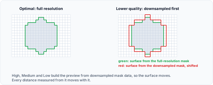
Generate an Optimal mesh preview now: click the green O button on the 3D view toolbar, or use View ▸ 3D View ▸ Mask 3D Preview (Mesh) ▸ Optimal and then the Mask 3D Preview (Mesh) button. You will need this preview again in Part 7.

Preview quality and measurements

High, Medium, and Low downsample the mask before the surface is generated, which shifts geometry slightly. Use Optimal whenever the preview feeds a measurement, an analysis, or an export.

Step 4.2: Recreate the material mask with Threshold

Model_Mask marks the solid material of the part. Build the same thing yourself with the parameters the tutorial script in Part 9 uses, so that you understand what each one does.

1. Go to Segmentation ▸ Create Mask ▸ Threshold.
2. Set the Lower Threshold to 31488 and the Upper Threshold to 65535. You can type the values, or drag the two lines on the histogram. Drag the shaded band between them to move the whole range without changing its width.
3. In Options, enable Fill cavities so that the internal voids are filled and the mask represents the solid body.
4. Enable Filter regions and choose Keep the largest region to discard fixture fragments and reconstruction noise.
5. In Result, leave the target mask on <New mask object> and the mode on Replace.
6. Click Apply.

Compare the new mask with Model_Mask in the slice views. Watch the live preview overlay while you move the thresholds: it is the fastest way to judge a threshold on an unfamiliar dataset.

Choosing a threshold from the data

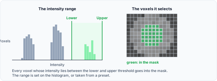
Expand the Profile line group, draw a line across a material boundary in a slice view, and read the intensity profile. The midpoint of the transition between air and material is a good first threshold.

Step 4.3: Edit the multi-label defect mask

Make Voids_Multilabel_Mask the active mask, then go to Segmentation ▸ Operations ▸ Multi-label Mask ▸ Multi-Label Mask Editor.

The Active mask labels table lists every label with its colour, its statistics, and its annotation. The group title shows the label count in brackets.

Try each operation:

1. Select two or three rows, right-click, and choose Combine. The selected labels are merged into one.
2. Select a row, right-click, and choose Remove. That label is deleted from the mask.
3. Right-click and choose Random Color or Custom Color... to recolour the selection.
4. Select several labels and click Create New Mask Object from Selected Label(s). The labels are extracted into a new mask object, leaving the original untouched.
5. Enable Show interactive annotation, then click a table row or pick a label in the 3D view. An annotation appears at that label's first voxel in every view.
6. Enable Show all labels annotations and choose 3D View or All Views in the adjacent list. All annotations are shown at once and repositioned automatically so they do not overlap.

Press Ctrl+Z to undo the combine and remove operations before you continue.

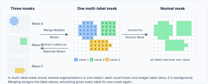
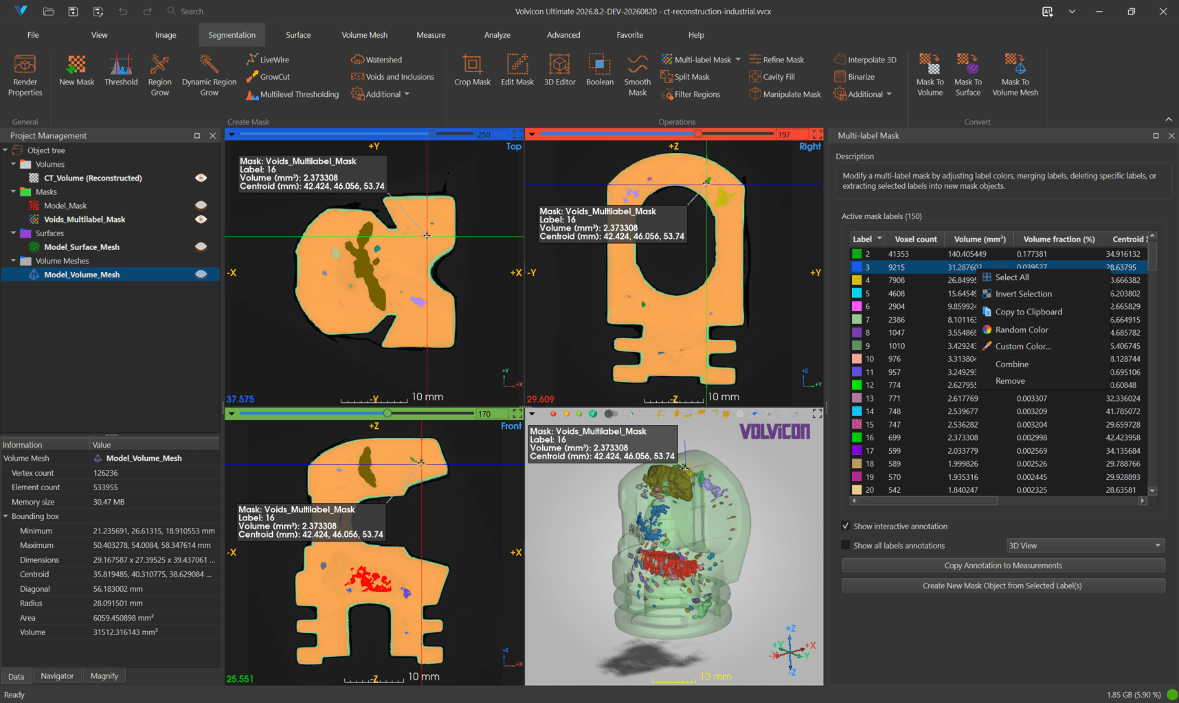
The same Multi-label Mask menu also offers Merge Multiple Masks, which builds one multi-label mask from several binary masks, Extract Labels as Separate Masks, which splits every label into its own object in one operation, and Convert to Normal Mask(s), which discards the label information. All four are pages of the same panel, so you can also switch between them in the Operations list at the top of the tool.

Step 4.4: The rest of the Segmentation tab

Section	Tools
Create Mask	New Mask, Threshold, Surface Determination, Region Grow, Dynamic Region Grow, Multilevel Thresholding, Watershed, Voids and Inclusions, and Additional with LiveWire and GrowCut
Operations	Crop Mask, Edit Mask, 3D Editor, Boolean, Smooth Mask, Multi-label Mask, Split Mask, Filter Regions, Refine Mask, Cavity Fill, Manipulate Mask, Interpolate 3D, Binarize, and Additional with Partial Volume Calculation, Invert Mask, Fill Holes, and Flip Mask
Convert	Mask To Volume, Mask To Surface, Mask To Volume Mesh

Two of them produce the kinds of object this project already contains: Voids and Inclusions creates a multi-label defect mask like Voids_Multilabel_Mask, and Mask To Surface creates a triangle mesh like Model_Surface_Mesh.

Step 4.5: Generate a surface from a mask

With your threshold mask active:

1. Go to Segmentation ▸ Convert ▸ Mask To Surface.
2. Set Target object(s) to Active mask object.
3. Set Quality to Custom so that all options become editable. With any other quality, the options are configured for you and cannot be changed.
4. Enable Resolution reduction and set XY resolution to 2.
5. Enable Smoothing and set Iterations to 50.
6. Enable Triangle reduction and set Reduction percent (%) to 80.
7. Click Apply.

These are the same settings the tutorial script in Part 9 uses, so the surface it builds matches the one you just made by hand.

---

Part 5: The Surface Tab, Repair Before You Measure

A surface generated from voxel data, or imported from another system, frequently contains defects that make Boolean operations, meshing, printing, and thickness measurement fail or return wrong numbers. Repair is therefore the first step, not a last resort.

Step 5.1: Run Diagnostics and Fixes

1. Make Model_Surface_Mesh active and visible.
2. Go to Surface ▸ Edit ▸ Diagnostics and Fixes.
3. On the Quick Fix tab, click Update. Volvicon reports the number of shells, overlapping triangles, intersecting triangles, holes, and inverted normals, plus the noise shell and non-manifold edge counts.
4. Review the fix options before you apply them. Unify, Remove small disconnected parts, Fix non-manifold edges, Separate repaired parts, Keep largest repaired part, and Force repair of unresolved non-manifold edges are all enabled by default, and several of them can remove geometry.
5. Click Fix, then Update again to confirm the counts improved.
6. Check the Comments section for the confirmation that the active surface mesh is closed and manifold.

Repairs can remove geometry

Remove small disconnected parts, Keep largest repaired part, and Force repair of unresolved non-manifold edges may delete valid detail. Duplicate an important surface before repairing it, and compare the result with the original.

Step 5.2: Work through the specialised tabs

Tab	What it gives you
Shells	A table of every disconnected component with its volume, area, and triangle count. Select rows to highlight them in 3D, then delete the ones you do not want.
Overlaps	Exact duplicate and zero-area triangles, highlighted in 3D and removable with Fix.
Triangles	Selection by intersection, non-manifold connection, area, angle, aspect ratio, or skewness, plus interactive Delete Triangle and Create Triangle modes.
Holes	Hole count with smallest and largest diameters, and Fill Holes.
Normals	Inverted triangle count, Fix Inverted Triangles, Invert All Triangles, interactive Invert Triangle, and Recompute Normals.

Hold Alt while an interactive mode is active to spin, pan, and zoom the camera without leaving the mode.

When one repair is not enough

Click Update after the first Fix. If the counts improved but issues remain, run Fix once more. If nothing changed, further repeats will not help, and you should inspect the highlighted area in the specialised tab or use Remesh.

Step 5.3: Cut the surface

The Cut tool removes or extracts part of the visible surfaces using region of interest (ROI) tools. Its description line states this directly: it uses basic, advanced, or primitive ROIs to cut the visible surfaces.

1. Hide every surface except Model_Surface_Mesh. The tool acts on all visible surfaces at once.
2. Go to Surface ▸ Edit ▸ Cut.
3. Set Operation to Retain. Cut deletes the selected region; Retain removes it from the original and creates a new surface object from it, which is safer while you are learning.
4. Set ROIs mode to Advanced, then choose the Cuboid ROI selection tool. Enable Show box, click Reset to fit the box to the bounding box of the visible surfaces, and then either drag its handles in the 3D view or type exact Position (mm), Size (mm), and Rotation (°) values.
5. Click Apply.

You now have two surface objects. The three ROI modes give you three ways to define the region:

Mode	Tools	How it applies
Quick	Rectangle, Polygon, Sphere, Plane, Cylinder, and Lasso, drawn directly in the 3D view	The operation runs as soon as you complete the ROI, so there is no Apply button
Advanced	Cuboid, Sphere, Cylinder, Plane, placed interactively and edited numerically	Reset fits the shape to the visible surfaces, Apply performs the cut
Primitives	A table of named ROI primitives, using the same shapes as the Primitives tool	Show the ROIs you want and click Apply to cut with all of them at once

Cutting leaves open boundaries. Use Surface ▸ Edit ▸ Fill Holes if you need the result to be closed again, or use Clip with its closed clip option when the cut must stay watertight from the start.

Step 5.4: The rest of the Surface tab

Section	Tools
General	Create, Render Properties
Transform	Transform, Interactive Transform, Global Registration
Edit	Diagnostics and Fixes, Merge, Split, Filter Shells, Editor, Cut, Clip, Boolean, Voxel Boolean, Fill Holes, Remesh, Voxel Remesh, Hollow, Smooth, Reduce, Subdivide, Extrude, Engrave Text, and an Additional menu with Mirror to Plane, Project to Plane, and Poisson Remesh
Analyze	Elevation, Surface Distance, Shortest Path, Collision Detection, Shells, Colorize
Convert	Surface To Mask, Surface To Volume Mesh

For an inspection workflow, the sequence that matters is Diagnostics and Fixes, then Remesh or Reduce to control triangle quality and count, then the analysis.

---

Part 6: The Volume Mesh Tab

A volume mesh fills the interior of a solid with tetrahedra so it can be simulated. Model_Volume_Mesh is the tetrahedral mesh of the part, and it is what you would hand to a solver.

Step 6.1: Inspect the mesh

1. Make Model_Volume_Mesh visible and active, and hide the volume and the masks.
2. Press E with the 3D view focused to switch to Solid Edges, or W for Wireframe, and inspect the element distribution.
3. Open Volume Mesh ▸ General ▸ Render Properties to set representation, material appearance, and bounding box display.
4. Read the Properties tab in the Project Management dock for the element and vertex counts, memory, and bounding box measurements.

Step 6.2: Generate your own volume mesh

1. Make a repaired, closed surface active.
2. Go to Surface ▸ Convert ▸ Surface To Volume Mesh.
3. Choose the algorithm and the output element type: Tetra 4-node (linear) for fast, large models, or Quadratic 10-node for stress analysis and curved boundaries.
4. When converting several surfaces at once, decide whether to maintain conformity so that shared interfaces get matching nodes.
5. Apply, and check the result with the mesh quality tools in Part 7.

Input quality decides success

Tetrahedralisation needs a closed, manifold, self-intersection-free surface with consistent outward normals. If the conversion fails or produces a poor mesh, go back to Diagnostics and Fixes rather than adjusting meshing parameters.

Step 6.3: The FEM tools

Tool	Purpose
Configure FEM Model	Define material properties, boundary conditions, and element sets
Export FEM Mesh	Write the configured mesh in a solver format

To bring a mesh back from a solver, use File ▸ Import ▸ Volume Mesh Models, or drag the solver file onto the 3D view. Where the file provides them, materials, node and element sets, surfaces, and parts are imported with the mesh.

Volume Mesh ▸ Convert ▸ Volume Mesh To Surface extracts the boundary surface again, which is a convenient way to check what a solver actually receives.

---

Part 7: The Measure Tab, Quantifying the Part

Step 7.1: Gray value statistics, whole volume and per slice

1. Make CT_Volume (Reconstructed) the active volume.
2. Go to Measure ▸ Statistics ▸ Volume Statistics.
3. Set Target to Active volume and Slice to All slices. The Whole volume statistics table reports mean, median, standard deviation, variance, minimum, maximum, sum, voxel count, skewness, and kurtosis.
4. Now set Slice to Current Plane 3 (XY) slice.
5. Scroll the mouse wheel in the blue Plane 3 (XY) slice view. The histogram and the statistics tables update as you move, so you are reading the gray value distribution of exactly the slice on screen.
6. Drag across the chart to mark a gray value range. The marked range reports its borders, mean, standard deviation, total, and share of the analysed data.
7. Set Target to Active mask with Model_Mask active to restrict the statistics to the material only, and compare the mean and standard deviation with the whole volume result.
8. Click Export... to write a CSV file or a PDF report.

CSV against report tables

The CSV export is written at the full resolution of the analysed region, so each row carries one gray value and its pixel count. The histogram table in the PDF report groups values into as many rows as the chart draws bars, and states the range each row covers. Use the CSV for further analysis and the report table to document what the chart shows.

Step 7.2: Per-label statistics for the defects

This is the core measurement for a porosity inspection.

1. Make Voids_Multilabel_Mask the active mask in the scene tree.
2. Go to Measure ▸ Statistics ▸ Mask Statistics ▸ Per-Label Mask Statistics.
3. Click the ... button next to Select statistics:. In the dialog, check Volume (mm³), Sphericity, Compactness, and Flatness, then click OK.
4. The statistics are computed and three tables are filled: Individual label statistics, Overall descriptive statistics, and Whole mask statistics.
5. Choose the metric to plot in Target metric:, pick a Lookup table:, and set the Number of bins: for the histogram.

The labels in the mask are recoloured from the selected lookup table according to the chosen target metric, so the largest, roundest, or flattest defects stand out immediately.

The 3D recolouring needs a 3D preview

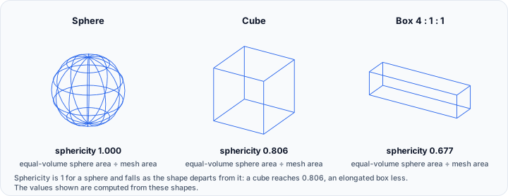
If the active multi-label mask has no valid 3D preview surface, the tables and the histogram are still computed, but the 3D preview is not recoloured and no colour scale is shown in the 3D view.

Generate the preview first: click the green O button on the 3D view toolbar, or use View ▸ 3D View ▸ Mask 3D Preview (Mesh) ▸ Optimal followed by the Mask 3D Preview (Mesh) button. Then reopen or re-run the statistics.

Finish with the annotations and the export:

• Enable Show interactive annotation and click a row to place an annotation at that defect in all views.
• Enable Show all labels annotations and select All Views to label every defect at once.
• Click Export... to produce a CSV file or a PDF report containing the settings summary, the tables, the histogram, the histogram data table, and optional snapshots and 3D scene.

The related tools are Whole Mask/Slice Statistics for aggregate numbers, Per-Region Mask Statistics for connected components of a binary mask, and the two 3D Preview variants that add surface area, mesh volume, vertex and face counts, and surface to volume ratio.

Step 7.3: Measurements

Create a measurement

1. Go to Measure ▸ Measurement tools ▸ Measurements.
2. Select a type from the list at the top: Point, Distance, Angle, Diameter, Contour, Circle, Ellipse, Rectangle, Box, or Caption.
3. Click the green + button at the bottom left of the table. Its tooltip reads "Add a new measurement." and it puts the views into placement mode.
4. Click in a 2D or 3D view to place the required points. For Distance that is two clicks, for Angle three with the vertex in the middle, and for Diameter three points on the circle. For Contour, left-click to add points and right-click to finish.
5. Grab a measurement handle and drag it. On a surface in the 3D view the handle follows the geometry, and the value updates live.

Read the table

The table has a Show column, a Lock column, a Name column, the measured value, and the point coordinates. Double-click the name cell to rename a measurement, and double-click a coordinate cell to type an exact position. Use the Lock column to protect a finished measurement from accidental dragging.

Right-click a row

Command	Effect
Select All / Invert Selection	Change the selection
Toggle Visibility / Isolate	Show or hide the selection, or hide everything else
Toggle Lock / Isolate Unlock	Lock or unlock the selection against editing
Locate	Centre every slice view on the selected measurement
Copy	Copy the selected rows to the clipboard
Duplicate	Create a copy of the selected measurements
Move Up / Move Down	Reorder the list
Remove Selected	Delete the selected measurements
Properties	Open the property dialog for name, colour, line width, font, and annotation content

The More options menu

The ... button next to the table opens the display options:

Entry	Effect
Always Show	Keep measurements visible after the tool is closed
Show In Slice Views	Draw measurements on the 2D views as well as in 3D
Annotation	Show On Active Only, Show All, or Hide All, and what the annotation contains: Name, Value, Name and Value, Position, or Name and Position
3D Axes	Show On Active Only, Show All, or Hide All for the 3D crosshair at each measurement
Handle	Show 2D Cross and Show Point control how handles are drawn
Surface	Snap To Surface... snaps the points of the selected measurement onto a surface
Properties...	The same property dialog as the context menu

Save and reload

Use Save and Load in the toolbar to export and import measurements as an INI file. Volvicon stores a SHA-256 integrity hash with the file and verifies it on import, warning you if the file was modified outside the application.

Primitives

Repeat the exercise in Measure ▸ Primitive tools ▸ Primitives, which creates reference geometry: Point, Line, Circle, Sphere, Ellipsoid, Cylinder, Capsule, Tube, Cone, Arrow, Spline, Plane, Cube, and Cuboid. Primitives use the same table, the same + button, and the same right-click and ... menus as measurements, and they can be positioned interactively with the 3D gizmo.

The Surface submenu of a primitive additionally offers Copy To Surfaces, which turns the selected primitives into real surface objects in the scene tree. That is the quickest way to get an exact analytical shape, a fitted sphere or cylinder for example, into the surface workflow.

Primitive Fitting fits primitives to existing geometry automatically, and Measurement between Primitives measures distances and angles between two of them.

Step 7.4: Mesh statistics and quality

• Measure ▸ Statistics ▸ Surface Statistics reports mesh statistics for Model_Surface_Mesh.
• Measure ▸ Statistics ▸ Volume Mesh Statistics does the same for Model_Volume_Mesh.
• Measure ▸ Analysis ▸ Mesh Quality Analyzer ▸ Surface Quality computes per-triangle metrics such as area, aspect ratio, condition, distortion, edge ratio, minimum and maximum angle, scaled Jacobian, and shape. Choose a Target metric, a Lookup table, and the Number of bins, then drag across the chart to quantify a range of elements before you adjust the thresholds. Volume Mesh Quality does the same for tetrahedra.

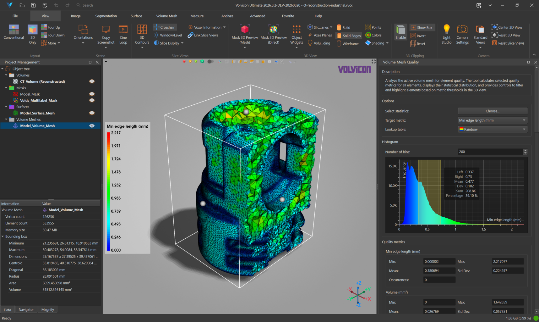
Also in the Measure tab: Histogram and Draw Profile Line in the measurement tools, Volume Similarity Statistics and Compare Masks in the statistics section, and Slice Analyzer in the analysis section. Every one of these offers Export..., which opens the PDF Report dialog described in PDF Report Generation.

---

Part 8: The Analyze Tab, Inspection Results

Every tool in this tab follows the same pattern: choose the analysis mode, create or load a named analysis, configure it, run it, then read the colour map, the histogram, and the statistics.

Step 8.1: Wall thickness on the part surface

1. Go to Analyze ▸ Analyses ▸ Wall Thickness Analysis and choose Analyze Surface.
2. Click Select analysis to open the Wall Thickness Analysis Editor.
3. Click New Analysis. A new row appears in the table.
4. Double-click the name and call it WallThickness_Model_Surface.
5. Set Actual Object to Model_Surface_Mesh.
6. Set Method to Ray casting, Max. Wall Thickness (mm) to 0 for an unlimited search, and leave Search Angle (deg) at 20, which the Shrinking sphere method uses.

7. Click Load to load the analysis and close the dialog. 8. Click Run Analysis.

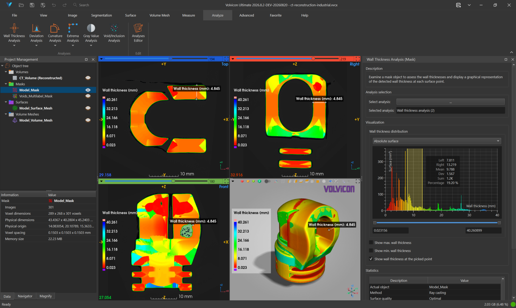
Read the result:

• The surface is coloured by thickness. Values below and above the visualisation range use their own dedicated colours.
• The Statistics table reports minimum, maximum, mean, standard deviation, surface area, surface area in range, and relative surface area in range.
• The histogram bars carry the colours of the colour map, so the chart and the coloured part can be read together.
• Show Minimum and Show Maximum annotate the extreme locations, and Pick Point reports the thickness wherever you click.
• Copy to Measurements transfers the visible annotations into the Measurements tool so they appear in measurement reports.

Isolating out-of-tolerance regions

Set the upper end of the visualisation range to your minimum acceptable wall thickness. Everything still coloured is at or below specification, and the Relative Surface Area in Range value tells you how much of the part that is.

Ray casting against Shrinking sphere

Ray casting projects along the surface normal in both directions and is fast and accurate where inner and outer walls are roughly parallel. Shrinking sphere searches a cone around the normal and handles curved, tapered, and non-parallel walls better at a higher computational cost. The two can select different opposing contacts, so for comparable inspections keep the method, maximum thickness, search angle, and mesh preparation identical across parts.

Step 8.2: Void and inclusion detection

1. Go to Analyze ▸ Analyses ▸ Void/Inclusion Analysis.
2. Click Select analysis, then New Analysis, and name it Voids_CT_Volume.
3. Set the Volume Object to CT_Volume (Reconstructed). Optionally set a Mask Object to restrict the search to the material, which speeds the analysis up and avoids boundary false positives.
4. Set Surface Quality to Optimal for a final result.
5. Click Edit Settings and configure the detection:
   • Mode: Void, which finds regions of lower intensity than the surrounding material.
   • Method: Absolute, with Auto absolute contrast enabled so the threshold is estimated from the data.
   • Auto air gray value enabled.
   • Under Filter Results, set a minimum size that excludes reconstruction noise. A minimum of about 27 voxels is a reasonable starting point for this dataset, and a minimum sphericity near 0.01 removes elongated streak artefacts.
6. Click Load, then Run Analysis.

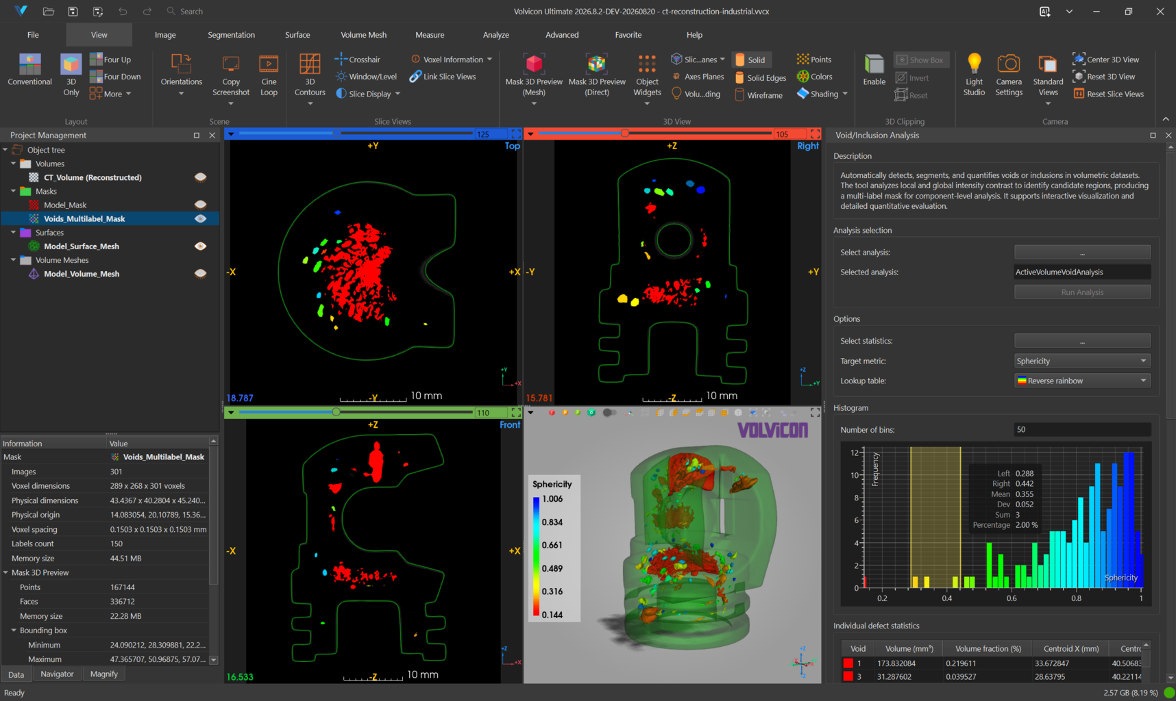
The analysis produces a multi-label mask in which each detected defect carries its own label, exactly like the shipped Voids_Multilabel_Mask. The statistics table lists per-defect volume, centroid, equivalent diameter, sphericity, compactness, surface area, and bounding box, and the summary reports total count, total volume, and volume fraction. Use Show all defect annotations with All Views to cross-reference the table against the viewport.

Step 8.3: The Analyses Editor

Open Analyze ▸ Edit ▸ Analyses Editor. It lists every analysis object stored in the project, grouped by type. The sample project ships with saved analyses from the session it was authored in, alongside the ones you just created.

Use the checkboxes and Select All / Deselect All to remove analyses you no longer need. This keeps a long-running inspection project readable.

Stored analyses reference objects by name

If an object was renamed after an analysis was created, the stored analysis still refers to the old name. Open the analysis in its editor and set Actual Object or Volume Object to the current object before running it again.

Step 8.4: The remaining analyses

Analysis	Use it for
Deviation Analysis	Comparing two objects point by point, for example a scan against a reference. Supports mask against mask, mask against surface, and surface against surface.
Curvature Analysis	Gaussian, mean, maximum, and minimum curvature on a surface.
Extrema Analysis	Local maxima and minima along a chosen direction vector.
Gray Value Analysis	Mapping volume gray values onto mask or surface geometry.

All of them export to CSV and to a PDF report through the same dialog.

---

Part 9: Automating the Workflow in Python

Everything in Part 5 and Part 8 can be scripted. The tutorial folder ships with a script that reproduces the threshold, surface generation, cleanup, and wall thickness workflow end to end.

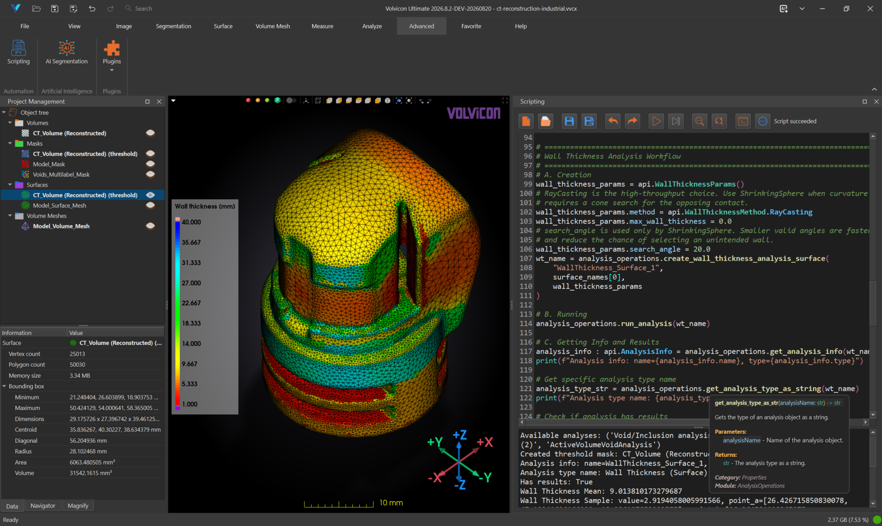
Step 9.1: Open the scripting editor

Go to Advanced ▸ Automation ▸ Scripting. The editor opens with a code pane, an output console, and a toolbar.

Step 9.2: Load the tutorial script

Click the toolbar button whose tooltip reads Load script from file, then select wall-thickness-analysis-script.py from your tutorial-1 folder.

Read through the script before running it. It performs the following steps:

1. Creates the application object, closes any open project, and opens ct-reconstruction-industrial.vvcx from the installation folder.
2. Prints the available analysis names and gets the active volume name.
3. Runs a threshold segmentation with a lower threshold of 31488 and an upper threshold of 65535, with cavity filling and largest-region filtering, which is exactly the operation from Step 4.2.
4. Converts the resulting mask to a surface with resolution reduction, 50 smoothing iterations, and 80 percent triangle reduction, which is exactly Step 4.5.
5. Remeshes and reduces the surface, then repairs it with the surface fixer.
6. Isolates the surface in the scene.
7. Creates a wall thickness analysis using the Ray Casting method, runs it, and prints the mean value plus the first few individual samples with their two contact points.
8. Writes the full result table to disk, changes the colour map and the visualisation range, saves three snapshots, and closes the project.

Edit the output paths first

The script writes its result file and its snapshots to C:\Samples\. If that folder does not exist on your machine, create it, or edit the four paths near the end of the script to a folder you can write to. Look for the write_wall_thickness_results_to_disk call and the three save_snapshot_to_disk calls.

The script also calls close_project() at the start and at the end, so save any work in the current project before you run it.

Step 9.3: Run it

Click the run button, or press Ctrl+R. Watch the output console: the script prints the created mask name, the analysis name and type, whether results exist, the mean wall thickness, and the first three samples with their coordinates.

Use Ctrl+Shift+R to stop a long-running script. Other useful editor shortcuts are Ctrl+/ to toggle comments, Ctrl+Alt+I to format indentation, Ctrl+Shift+F to find, and Ctrl+Shift+H to find and replace. The Insert code templates button adds ready-made snippets for common workflows.

Step 9.4: Understand the boundary between script and interface

The script header states the trade-off plainly, and it is worth internalising. Interactive analysis relies on picking points, reading charts, and adjusting ranges by eye, none of which a script can do. Scripting is therefore the right tool for repeatable batch work, and the Analyze tab is the right tool for investigation and for report generation with snapshots, measurements, interactive 3D scenes, and charts.

To go further, see Python Scripting Fundamentals, Batch Processing and Automation, and the API Reference.

---

Part 10: Recording a Presentation Video

The last deliverable of an inspection is often a video. The tutorial folder ships with a complete timeline you can import.

Step 10.1: Prepare the scene

The animation drives objects by role, not by name, so the right objects have to exist and be visible before you start:

1. Make Model_Surface_Mesh visible.
2. Make Voids_Multilabel_Mask visible and generate its 3D preview at Optimal quality using the green O button on the 3D view toolbar.
3. Make CT_Volume (Reconstructed) visible, since the timeline fades the active volume.
4. Leave the camera as the project restored it. The enabled camera path track in this preset was authored on this exact scene, so its keyframes already frame the part correctly.

Step 10.2: Open the Video Recorder and import the timeline

1. Open File ▸ Media ▸ Record Video, or press Ctrl+Alt+R. The recorder docks at the bottom of the window.
2. In Capture, set the target to 3D view for a clean render, or Application if you want the whole interface in the video.
3. Set Animation to Timeline (tracks).
4. Click Presets ▸ Import from File... and select video-recorder-animation-preset.json. Confirm replacing the current tracks.

Step 10.3: Read the timeline

Seventeen tracks appear on the shared time axis, running to a total of about 19.3 seconds. Fourteen are enabled and three are switched off, ready as alternatives.

Time	What happens	Track types
0 s to 6 s	The active volume fades away, the surfaces are held hidden, the third slice plane sweeps forward through the part while its plane fades out in 3D, and a clipping sweep opens all masks along Z	Opacity fade, Slice sweep, Clipping sweep
0 s to 9 s	A smooth camera path carries the viewpoint through the first half of the sequence	Camera path
6 s to 12 s	The slice sweeps back, a reversed clipping sweep reveals all surfaces, the masks fade out, the surfaces are held at full opacity, and the volume finishes fading	Slice sweep, Clipping sweep, Opacity fade
9 s to 19.3 s	A horizontal camera orbit makes one full turn around the part	Camera orbit
15.3 s to 19.3 s	The surfaces fade out over 1 second, the masks over 4 seconds, closing the sequence	Opacity fade

Three tracks are imported disabled: a neutral studio background fade and two alternative camera paths. Click the small indicator on the left of a track bar to enable or disable it.

About the two disabled camera paths

A camera path track stores absolute viewpoints. The enabled path was recorded on this project, so it frames the part correctly. The two disabled paths were authored on a different scene and will point the camera somewhere else if you switch them on. Enable one, select it, and use Update on each keyframe to re-capture it from the current camera if you want to reuse its timing on this part.

Work with the timeline directly:

• Drag a bar to change its start time, and drag its left or right edge to change its duration.
• Select a track to edit its settings in the panel on the right, or type exact values into the Start and Duration boxes below the timeline.
• Zoom with Ctrl and the mouse wheel, or with the -, +, and Fit buttons.
• Double-click a track to rename it, and right-click for Enabled, Duplicate, Remove, Move Up/Down, Start at Zero, Snap to Previous Track End, and Expand to Timeline End.

Step 10.4: Preview and record

1. Click Preview. An orange playhead sweeps the timeline and the animation plays in the view without writing a file.
2. If a message reports that no object matches an opacity track, the required objects are not visible. Go back to Step 10.1, make them visible, regenerate the mask preview, and preview again.
3. Click Settings... to set the Frame rate (30 fps suits most presentations), the Quality preset, the Format (MP4 with H.264, AVI with H.264, or AVI with Motion JPEG), and the output Folder. When the folder is empty, videos go to your Videos folder.
4. Click Record. The animation is rendered frame by frame, so the duration and smoothness are exact regardless of how fast your computer is.
5. When recording finishes, the saved file name is shown in the toolbar, with the full path in its tooltip.

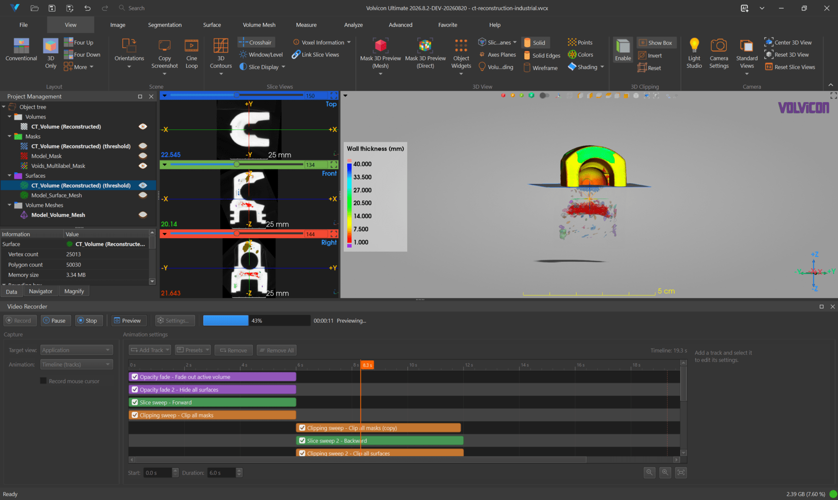
Every camera, opacity, clipping, slice, and background state is restored when the recording or preview ends, so the scene you return to is the one you left.

Build a reusable library

Click Presets ▸ Export to File... to save your adjusted timeline. Because tracks reference objects by role rather than by name, the same file produces the same animation on any comparable project. Camera path tracks store absolute viewpoints, so re-frame the scene after importing onto a differently sized part.

---

What You Have Built

By the end of this tutorial you have:

• Rendered a 16-bit industrial CT volume with a custom transfer function and isosurface.
• Reproduced the material segmentation from its threshold parameters.
• Edited a multi-label defect mask and extracted labels into new objects.
• Repaired a triangle mesh and verified that it is closed and manifold.
• Measured gray values per slice and per mask, and defects per label.
• Run wall thickness and void analyses and exported their results.
• Executed the same workflow unattended from a Python script.
• Composed and recorded a multi-track animation of the finished scene.

---

Next Steps

Direction	Where to go
Medical imaging workflows	Tutorial 2: Medical CT, From AI Segmentation to Simulation
Importing your own scans	Tutorial 3: DICOM Import and Semi-Automatic Segmentation
More on inspection analyses	Quality Analysis
More on automation	Batch Processing and Automation
Reference for any tool used here	GUI Reference