Tutorial 3: DICOM Import and Semi-Automatic Segmentation

This tutorial starts where every clinical project starts: with a folder of DICOM files. You will import the sample series, verify that it arrived correctly, and then work through the four segmentation families that Volvicon offers for intensity-based data, ending with a refined, named mask and a surface model.

Estimated time: 45 minutes

Level: Beginner to intermediate

Dataset: samples\tutorial-data\DICOM-1

Medical Use Disclaimer

Volvicon is not a regulated medical device. It has not been cleared by the FDA, CE marked, or approved by any other regulatory body for clinical diagnosis, treatment planning, or medical decision making. You are responsible for compliance with local privacy regulations, appropriate handling of protected health information, application of anonymisation where required, and validation of results before any clinical use.

---

What You Will Learn

1. Import a DICOM series, review its metadata, and control anonymisation.
2. Verify geometry and gray values after import.
3. Segment with a two-sided Threshold, a one-sided Surface Determination, and automatic Multilevel Thresholding.
4. Segment a connected structure with Dynamic Region Grow, then extend it in Merge mode.
5. Refine, name, and convert the result.

---

The Dataset

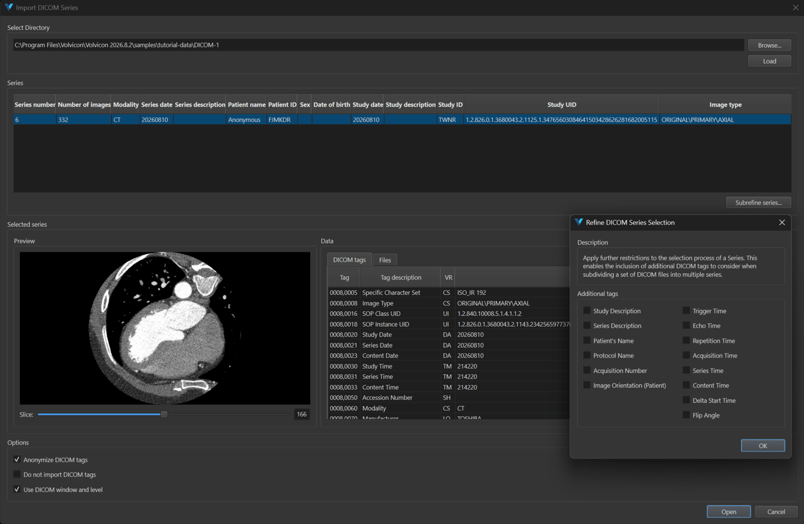
DICOM-1 contains a single anonymised CT series exported as 332 individual files, IMG0001.dcm through IMG0332.dcm.

Property	Value
Modality	CT
Files in series	332
Series number	6
Image type	ORIGINAL, PRIMARY, AXIAL
Matrix per slice	512 x 512
Pixel spacing	0.429 x 0.429 mm
Slice increment	0.3 mm
Reconstruction diameter	220 mm
Body part examined	HEART
Scan options	HELICAL_CT
Tube voltage / current	120 kVp / 500 mA
Stored window centre / width	120 / 700
Patient name / ID	Anonymous / FJMKDR

After import the volume is 512 x 512 x 332 voxels, roughly 220 x 220 x 100 mm.

Hounsfield units

The series has a rescale slope of 1 and a rescale intercept of 0, so the stored values are Hounsfield units. Air reads around -1000, fat around -100, muscle and other soft tissue between roughly 20 and 80, contrast-enhanced blood a few hundred, and bone and calcification above roughly 300. Regions outside the reconstructed field of view are padded at -2048, which is why the histogram has a tall spike at its lower end.

---

Part 1: Importing the Series

Step 1.1: Open the DICOM Import dialog

Go to File ▸ New ▸ DICOM Images.

Use File ▸ Import ▸ DICOM Images instead when you want to add a series to the project you already have open. New clears the scene first and prompts you to save unsaved changes.

Step 1.2: Scan the folder

1. Click Browse... next to Select Directory and select your copy of the DICOM-1 folder.
2. Click Load. Volvicon scans the folder and its subfolders and groups the files into series.

One row appears in the Series table. Check these columns against the dataset:

Column	Expected value
Series number	6
Number of images	332
Modality	CT
Series date / Study date	The acquisition date recorded in the files
Patient name	Anonymous
Patient ID	FJMKDR
Study ID	TWNR
Image type	ORIGINAL\PRIMARY\AXIAL

The Series description and Study description columns are empty for this dataset, because those tags are not present in the files. That is normal for exported and anonymised data.

If no series is detected, confirm that you selected the folder that contains the files, not a parent two levels up, and that the files are valid DICOM.

Step 1.3: Preview the slices

Click the series row to select it, then drag the Slice: slider from the first slice to the last, or type a slice number into the spin box next to it. The preview uses the DICOM window and level values from the series, so it looks the way a DICOM viewer would show it.

Scrolling the whole series before importing is worth the thirty seconds. It catches truncated transfers, mixed acquisitions, and wrong-orientation exports before they become a segmentation problem.

Step 1.4: Inspect the metadata

The Data group below the preview has two tabs describing the selected series:

• DICOM tags lists the metadata in a Tag, VR, Tag description, and Value table: patient information, modality, pixel spacing, slice thickness, and the default window centre and width.
• Files lists every file that makes up the series with its full Path, which confirms that the expected files were grouped together.

Step 1.5: Set the import options

Option	Default	Effect
Anonymize DICOM tags	Enabled	Removes identifying tags from the metadata stored in the project
Do not import DICOM tags	Disabled	Imports pixel data only, with no metadata at all. Disables the anonymisation option, because there is nothing left to anonymise
Use DICOM window and level	Enabled	Applies the window centre and width from the series to the imported volume. With it disabled, Volvicon computes values from the actual intensities

Leave the defaults for this tutorial.

What anonymisation does and does not do

Anonymisation removes identifiers from the DICOM tags stored in the project file. It does not remove burned-in annotations from the pixel data, it does not change the original files on disk, and it does not by itself guarantee complete de-identification for every use case. In a regulated environment, validate that your requirements are actually met.

Disabling anonymisation shows a privacy warning. Only disable it when you have explicit authorisation to retain identifiable information.

Step 1.6: Refine the series if needed

Some folders contain several phases, orientations, or acquisition parameters that share one Series Instance UID. Click Subrefine Series... and add separation criteria such as Series Description, Acquisition Number, Image Orientation (Patient), Trigger Time, Echo Time, or Acquisition Time. The table is re-analysed and the mixed series splits into distinct rows.

DICOM-1 is a single clean series, so no refinement is needed here.

Step 1.7: Import

Click Open. The volume appears in the scene tree and the views fill with the imported data.

Multi-frame time sequences

When several series share compatible geometry, you can Ctrl-click to select them all and import them as time frames of one 4D volume, then review them with View ▸ Scene ▸ Cine Loop. See DICOM Import.

---

Part 2: Verifying and Preparing the Volume

Step 2.1: Check the geometry

Open the Properties tab in the Project Management dock and compare the reported slice count, voxel grid, physical dimensions, spacing, and gray value range with the dataset table above. Every millimetre result you produce later depends on these numbers being right.

Step 2.2: Set a medical orientation

Go to View ▸ Scene ▸ Orientations and select Medical 1 or Medical 2. The axis labels change to Left, Right, Anterior, Posterior, Superior, and Inferior, and the slice views are named Plane 1 (YZ), Plane 2 (XZ), and Plane 3 (XY). The preset changes labelling only, never the voxel data.

Matching another application's layout

If you need the display to match a RAS-based application such as 3D Slicer, use Image ▸ Transform ▸ Flip to flip X and then Y, each with Flip Reference set to About origin. This one does change the voxel data, so verify left and right anatomy afterwards. Use Swap Axes instead when the axes are permuted rather than inverted.

Step 2.3: Set the contrast

1. Open View ▸ Slice Views ▸ Window/Level.
2. Select CT-Bone (level 400, window 1000) from the Presets list, then CT-Abdomen (level 40, window 350), then Blood (level 100, window 600). Watch which structures each one brings out.
3. Drag either boundary line on the histogram to change the window, and drag the shaded band between them to change the level.
4. With the panel open, drag with the left mouse button in a slice view: horizontally for the window, vertically for the level.

Window and level change the display only. They never modify the image data, and they never affect a threshold.

Step 2.4: Turn on the readouts you will need

1. Enable Crosshair from the slice view context menu. Middle-click to move it, or hold Alt and move the mouse for continuous tracking.
2. Set Voxel Information to Both.
3. Hover over air, fat, muscle, contrast-filled blood, and bone in turn, and read the HU value for each. Write down the values you see. Those numbers, not textbook values, are the ones your thresholds should be built on.

---

Part 3: Threshold Segmentation

Thresholding classifies each voxel purely by its intensity. It is the fastest segmentation method and the right first choice whenever the target structure has a distinct intensity range.

Step 3.1: Two-sided threshold

1. Go to Segmentation ▸ Create Mask ▸ Threshold.

2. Open the Presets list. Each entry shows a thumbnail rendered from the current volume, so you can compare them visually. The supplied presets are calibrated for Hounsfield units:

   Preset	Range (HU)
   Bone	226 to 10000
   Muscle	-5 to 135
   Fat	-205 to -51
   Skin	-718 to -177
   Tooth	1200 to 10000

3. Select Bone. The thresholds are applied and the preview overlay appears in the slice views.

4. Fine-tune the range: drag either threshold line on the histogram, drag the shaded band between them to move the range without changing its width, or type exact values. Hold Ctrl and scroll the wheel over the chart to zoom into a narrow band of gray values.

5. In Options, decide what to clean up:

   Option	Effect
   Fill cavities	Fills internal gaps so the mask represents a solid body
   Filter regions ▸ Keep the largest region	Keeps only the largest connected component
   Filter regions ▸ Remove regions	Removes components below Minimum region size (voxels)

6. In Result, leave the target mask on <New mask object> and the mode on Replace.

7. Click Apply.

Step 3.2: Find a threshold from the data

When no preset fits, read the value off the image instead of guessing:

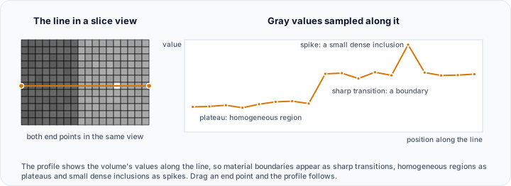
1. Expand the Profile line group.
2. Draw a line in a slice view that crosses the boundary you care about, for example from soft tissue into bone.
3. The chart shows the intensity profile along that line. The midpoint of the transition is a good starting threshold.
4. Adjust the threshold lines on the histogram and watch the preview overlay until the boundary sits where you want it.

Save your own preset

Once you have a range that works for a class of studies, save it as a preset from the preset widget. Presets are stored per user, so they follow you across projects.

Step 3.3: One-sided threshold with Surface Determination

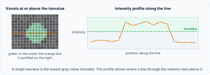
When a single value separates the material from everything below it, Surface Determination is simpler and has one fewer parameter to get wrong. It also places that surface between voxels rather than on them, so the mask can be measured afterwards.

1. Go to Segmentation ▸ Create Mask ▸ Surface Determination.
2. Leave Method on ISO50. The tool reads the gray value distribution of the volume and fills in the background, the material and the resulting Isovalue.
3. Read Separation in the Gray values group. Above 3 the two populations are well apart from the noise.
4. To choose the value yourself, set Method to Manual and type it into Isovalue, or drag the line on the histogram. Everything at or above the isovalue is material.
5. Use the Profile line group as in Step 3.2 if you need to justify the value.
6. Choose the target mask in Result, then click Apply.

Cavity filling and region filtering are separate mask tools. Apply them afterwards if you need them, keeping in mind that they change the determined surface.

Tool	Bounds	Use it when
Surface Determination	One lower bound	One value separates your material from everything below it
Threshold	Lower and upper bound	Both ends of the included range matter, for example soft tissue between air and bone
Multilevel Thresholding	Automatic, several thresholds	You want the data itself to propose the class boundaries

Step 3.4: Automatic multilevel thresholding

1. Go to Segmentation ▸ Create Mask ▸ Multilevel Thresholding.

2. Set Target object(s) to Active volume object.

3. Choose the Thresholding method:

   Method	How it decides
   Otsu	Selects thresholds that maximise the variance between the resulting classes. Best when the histogram has clear, separate peaks.
   K-means	Clusters voxel intensities and uses the cluster centroids as thresholds. More flexible when the peaks overlap.

4. Set Number of masks to 3 to separate air, soft tissue, and dense structures. The range is 1 to 999, and the default is 2.

5. Click Apply.

One mask object is created per class. Review them in the slice views, delete the ones you do not need, and rename the rest.

When automatic thresholding disappoints

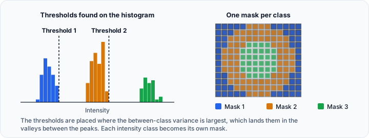
Multilevel thresholding works from the histogram alone. If two structures share an intensity range, no threshold can separate them, and no setting in this tool will change that. Move on to region growing, or combine a coarse threshold with a spatial method.

---

Part 4: Dynamic Region Grow

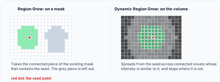
Thresholding takes every voxel in range anywhere in the volume. Region growing takes only voxels that are connected to a point you choose, which is what you want for a single organ, a vessel tree, or one bone among several with the same density.

Step 4.1: Configure the tool

1. Go to Segmentation ▸ Create Mask ▸ Dynamic Region Grow.

2. Set Region growing method to Connectivity. Rather than using a fixed intensity range, this method records the intensity statistics around the seed and includes neighbouring voxels that match them.

3. Enter the parameters:

   Parameter	Value	Meaning
   Multiplier	2	Width of the confidence interval for intensity similarity. Higher values grow further and leak sooner.
   Number of iterations	2	How often the filter re-estimates the statistics and grows again.
   Initial neighborhood radius (pixels)	2	Size of the neighbourhood sampled around the seed.

4. In Options, leave Multiple layer checked so the region grows through the whole volume. Unchecked, it is confined to the current slice.

5. In Result, leave the target mask on <New mask object> and the mode on Replace.

Step 4.2: Place the seed

Left-click on the structure you want in any 2D or 3D view. The region grows from that point immediately and is written to a new mask object.

In the 3D view, hold Ctrl and drag to rotate the camera while the tool is active, so you can reach a face that is currently turned away.

Check the result in all three slice views:

Symptom	Fix
The region leaked into a neighbouring structure	Undo with Ctrl+Z, reduce the Multiplier, seed again
The region stopped far short of the structure	Increase the Multiplier or the Number of iterations
The region is noisy at the edges	Increase the Initial neighborhood radius, or clean up afterwards with Smooth Mask

Seed placement decides the outcome

Everything the algorithm does follows from the statistics it measures at the seed. Place it in a homogeneous, representative part of the structure, away from partial-volume boundaries and away from metal or beam-hardening artefacts.

Step 4.3: Name the mask

Rename the new mask before you forget what it is:

• Double-click its name in the scene tree and type a new one, or
• Right-click it and choose Rename.

Duplicate names are adjusted automatically so every object stays uniquely identifiable.

Step 4.4: Add the regions that were missed

A single seed rarely captures everything. Extend the same mask rather than accumulating a pile of fragments:

1. In the Dynamic Region Grow panel, select your renamed mask in the Result target mask list.
2. Select the Merge radio button. Replace would overwrite what you already have; Merge adds to it.
3. Click on a missing region in a slice view. The newly grown region is merged into the existing mask.
4. Repeat for each missing part, checking the result after every click.

Each click is a separate operation, so Ctrl+Z removes only the last addition and leaves the rest of your work intact.

Step 4.5: The threshold variant

Switching Region growing method to Threshold gives you a different trade-off: the region grows from the seed but includes only voxels inside an explicit intensity range that you set on the histogram, using either 6-connectivity (face neighbours only, more conservative) or 26-connectivity (faces, edges, and corners, better through thin connections).

Use it when you already know the intensity range of the target and want strict control over it. Use Connectivity when you would rather let the data around the seed decide.

---

Part 5: Refining and Finishing

Step 5.1: Correct by hand

Open Segmentation ▸ Operations ▸ Edit Mask:

Tool	Use
Brush	Paint or erase freehand. Left-click and drag.
Rectangle, Circle, Lasso	Left-click and drag, release to apply.
Polygon	Left-click to add vertices, middle-click to close and apply.
LiveWire	Semi-automatic edge tracing along image boundaries.
Level Tracing	Intensity-based boundary tracing, left-click and drag.

Shortcut	Action
Shift (hold)	Temporarily switch from Draw to Erase
+ / -	Increase or decrease the brush size
Ctrl+Shift+B	Toggle the brush shape between Circle and Rectangle

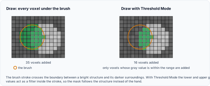
Enable Threshold mode with Draw to restrict painting to voxels inside a gray value range. You can then sweep the brush roughly over bone without picking up the surrounding soft tissue.

For editing directly in 3D, use Segmentation ▸ Operations ▸ 3D Editor.

Step 5.2: Clean up with the mask operations

Tool	What it fixes
Smooth Mask	Jagged borders, using a discrete gaussian, recursive gaussian, mean, or median filter
Cavity Fill	Cavities enclosed inside the structure
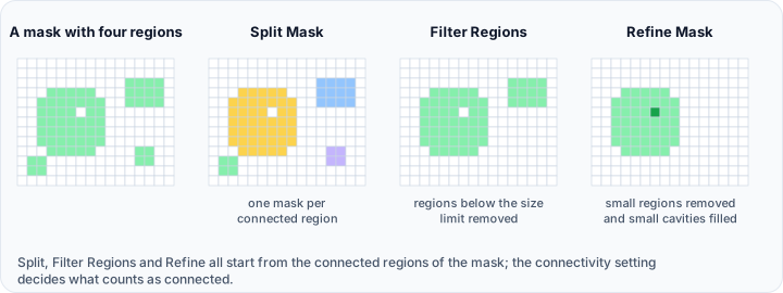
Filter Regions	Small disconnected specks, or oversized regions
Refine Mask	Artifacts and small holes in one pass
Manipulate Mask	Hollow, grow, or shrink the boundary
Interpolate 3D	Gaps left when you segmented only every few slices
Split Mask	Disconnected regions that belong in separate objects
Boolean	Union, intersection, or difference against another mask
Crop Mask	Content outside a bounding box

Segment every few slices, then interpolate

For a structure with a smoothly changing cross-section, trace every third or fourth slice with LiveWire or the brush, then run Interpolate 3D. It is usually faster than tracing every slice and the result is smoother.

Step 5.3: Check your work in 3D and in numbers

1. Make the mask visible and click the green O button on the 3D view toolbar to generate a Mask 3D Preview (Mesh) at Optimal quality.
2. Turn on View ▸ Slice Views ▸ 3D Contours ▸ Mask(s) Preview. The intersection of the preview with each slice is drawn on the 2D views, which is the quickest way to spot a boundary that drifted.
3. Open Measure ▸ Statistics ▸ Mask Statistics ▸ Whole Mask/Slice Statistics and read the volume, surface area, and intensity statistics of the result.
4. If you segmented the same structure twice with different methods, compare them with Measure ▸ Statistics ▸ Compare Masks.

Step 5.4: Convert the mask

Target	Tool	Purpose
Triangle mesh	Segmentation ▸ Convert ▸ Mask To Surface	Visualisation, export, 3D printing, surface analysis
Tetrahedral mesh	Segmentation ▸ Convert ▸ Mask To Volume Mesh	Simulation
Grayscale volume	Segmentation ▸ Convert ▸ Mask To Volume	Further image processing on the segmented region

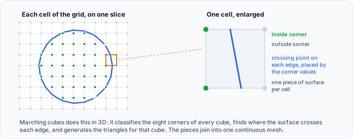
After Mask To Surface, always run Surface ▸ Edit ▸ Diagnostics and Fixes before any measurement, Boolean operation, meshing, or export. A surface extracted from a segmentation is rarely free of holes, non-manifold edges, or inverted normals.

Step 5.5: Save the project

Press Ctrl+S, or use File ▸ Save As to write a new .vvcx project. The project stores the volume, every mask, surface, and volume mesh, all render settings, the camera, the analyses, and an integrity manifest that is verified the next time the project is opened.

To hand individual objects to another application instead, use File ▸ Export, or right-click the object in the scene tree and choose Export.

---

Troubleshooting

Problem	Cause	What to do
No series detected after Load	The folder holds no valid DICOM files, or you selected the wrong level	Verify the folder, and try the parent folder if the files sit in subfolders
Series look mixed or incorrect	Several acquisitions share one Series Instance UID	Use Subrefine Series... to add separation criteria
Import fails on a large series	Not enough memory, missing read permission, or a corrupt file	Check available memory and permissions, and look for damaged files
The preview orientation looks wrong	Display convention, not data	Change the Orientations preset, or flip X and Y about the origin to reach RAS
Threshold selects the wrong tissue	The window and level were mistaken for the threshold	Window and level affect display only. Read real HU values with Voxel Information and set the threshold from those
The mask has a spike of voxels at the image border	Padding outside the reconstructed field of view is stored at -2048	Keep the lower threshold above the padding value, or crop the volume first
Region growing leaks everywhere	The Multiplier is too high, or the seed sits on a boundary	Lower the multiplier and re-seed inside a homogeneous area
The 3D preview does not appear	The mask is not visible, or no preview was generated	Make the mask visible, then generate the preview at Optimal quality

---

What You Have Built

• An imported, anonymised CT volume with verified geometry and calibrated gray values.
• Masks created with two-sided thresholds, a one-sided isovalue, and automatic class separation.
• A connected structure segmented from a seed point and extended in Merge mode.
• A refined, correctly named mask, converted to a repaired surface.
• A saved project that reopens with everything intact.

---

Next Steps

Direction	Where to go
Continue with a full anatomical workflow	Tutorial 2: Medical CT, From AI Segmentation to Simulation
Industrial inspection workflows	Tutorial 1: Industrial CT Inspection
More on thresholds	Threshold Segmentation
More on region-based methods	Region-Based Segmentation
More on manual correction	Manual Mask Editing
Reference for any tool used here	GUI Reference