Void/Inclusion Analysis

The Void/Inclusion Analysis tool automatically detects, segments, and quantifies internal voids (porosity) or inclusions within volumetric datasets. This analysis is essential for non-destructive testing (NDT), quality control, and material characterization workflows where identifying and measuring internal defects is critical.

Understanding Void and Inclusion Detection

The analysis examines local and global intensity contrast within the volume data to identify regions that differ from the surrounding material. Voids appear as lower-intensity regions (typically air or gas pockets), while inclusions appear as higher-intensity regions (denser foreign materials).

The tool produces a multi-label mask where each detected defect is assigned a unique label, enabling individual defect characterization. Statistical analysis provides measurements for each defect (volume, location, shape metrics) as well as aggregate statistics for the entire analysis.

Industrial Applications

Void/Inclusion Analysis is commonly used in:

• Casting inspection: Detecting porosity, shrinkage, and gas pockets
• Additive manufacturing: Identifying lack-of-fusion defects and voids
• Composite materials: Locating delamination and inclusions
• Welding inspection: Finding porosity and slag inclusions

Accessing the Tool

1. Navigate to the Analyze ribbon tab.
2. Click the Void/Inclusion Analysis button.
3. The tool opens with the analysis controls panel.

Analysis Configuration

Creating a New Analysis

1. In the Analysis Selection section, click Select analysis to open the Void/Inclusion Analysis Editor dialog.
2. Click New Analysis to create a new analysis configuration.
3. Configure the analysis parameters:
   • Select the Volume Object to analyze
   • Optionally select a Mask Object to restrict analysis to a specific region
   • Set the Surface Quality for visualization
   • Click Edit Settings to configure detection parameters
4. Click Load to load the selected analysis and close the dialog.

Editor Dialog Parameters

Parameter	Description
Analysis Name	User-defined name for the analysis.
Volume Object	The volume image to analyze for defects.
Mask Object	Optional multi-label mask for results (or to use existing results).
Surface Quality	Quality of 3D preview for detected defects: Optimal, High, Medium, or Low.
Analysis Settings	Opens the detailed settings dialog for detection parameters.

Detection Settings

Click Edit Settings to access the detailed analysis parameters:

Analysis Type

Parameter	Options	Description
Mode	Void, Inclusion	Void detects lower-intensity regions (porosity); Inclusion detects higher-intensity regions (dense materials).
Method	Absolute, Relative	Absolute uses fixed contrast thresholds; Relative uses percentage-based thresholds.

ROI Mask

Parameter	Description
Mask Object	Optional mask to restrict analysis to a specific region of interest.

Analysis Parameters

Parameter	Description
Auto absolute contrast	Automatically estimate the absolute contrast threshold based on data statistics.
Absolute contrast	Manual threshold for absolute intensity difference from surrounding material.
Relative contrast (%)	Percentage-based contrast threshold relative to local intensity range.
Auto air gray value	Automatically estimate the gray value representing air/void.
Air gray value	Manual specification of the intensity value representing air or void.

Filter Results

Configure filters to refine which detected regions are included in the final results:

Parameter	Description
Probability threshold	Minimum confidence score for including detected regions (0.0–1.0).
Min. size	Minimum defect size (volume in mm³ or voxel count).
Max. size	Maximum defect size (volume in mm³ or voxel count).
Compactness range	Filter by compactness metric (0.0–1.0). Higher values indicate more compact shapes.
Sphericity range	Filter by sphericity (0.0–1.0). Values near 1.0 indicate sphere-like shapes.
Volume fraction range	Filter by defect volume as percentage of total analyzed volume.
Equivalent diameter range	Filter by equivalent spherical diameter (mm).
Max. count	Maximum number of defects to include in results.

Running the Analysis

1. After loading an analysis configuration, click Run Analysis.
2. A progress dialog appears while the analysis:
   • Segments candidate defect regions
   • Applies filtering criteria
   • Generates the multi-label mask
   • Calculates statistics for each defect
3. Upon completion:
   • Detected defects are displayed as colored regions in 3D and 2D views.
   • The statistics table populates with per-defect measurements.
   • The histogram shows the distribution of the selected metric.

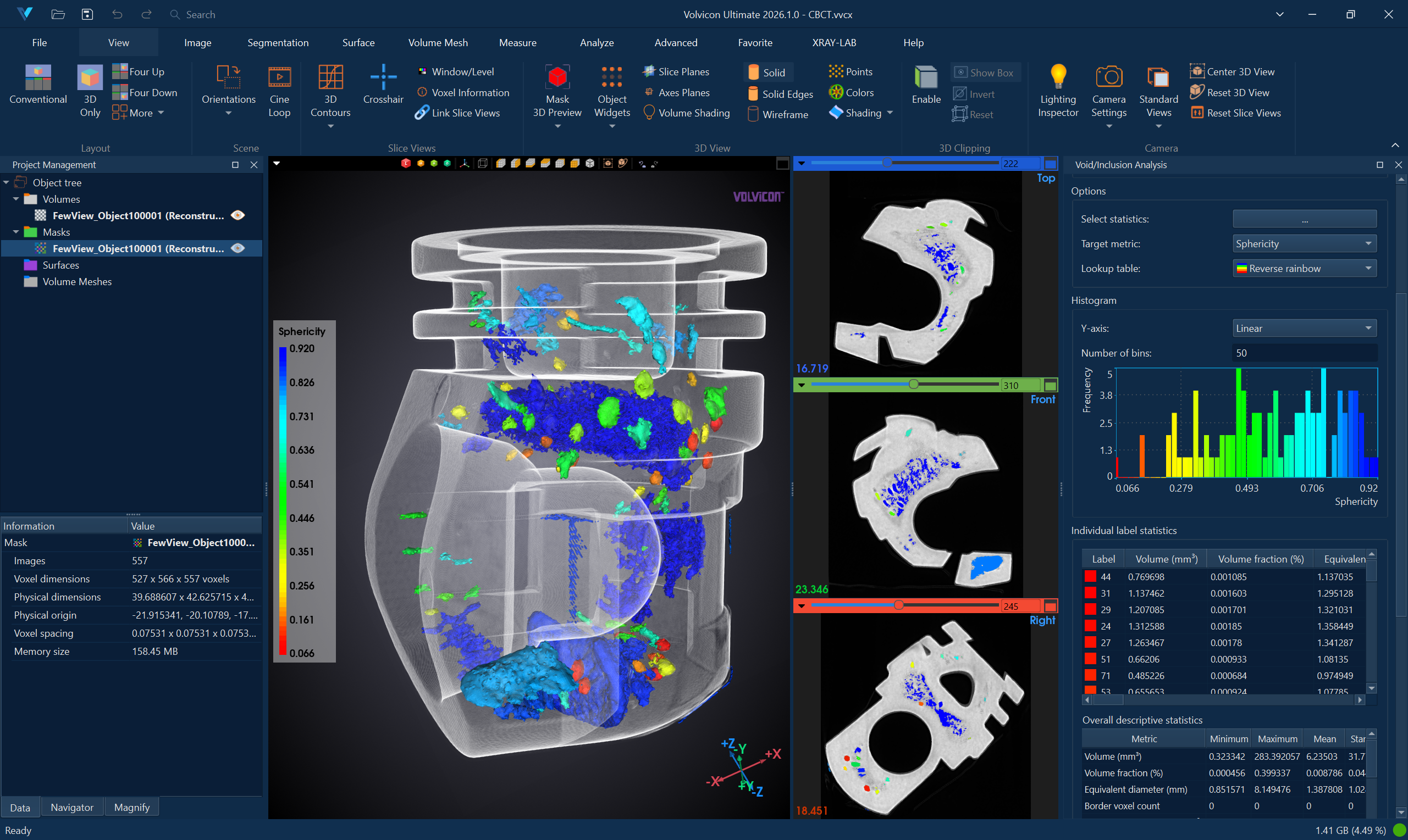
Interpreting Results

Visualization

Each detected defect is displayed as a distinct colored region:

• Individual defects are assigned unique colors for easy identification
• The 3D view shows the spatial distribution of all detected defects
• 2D slice views show defect cross-sections at each slice location

Statistics Table

The analysis provides detailed per-defect statistics:

Statistic	Description
Label	Unique identifier for each detected defect.
Volume (mm³)	Physical volume of the defect.
Centroid X, Y, Z	Spatial coordinates of the defect center.
Equivalent Diameter (mm)	Diameter of a sphere with equivalent volume.
Sphericity	How closely the defect resembles a sphere (0.0–1.0).
Compactness	Measure of how compact the defect shape is (0.0–1.0).
Surface Area (mm²)	External surface area of the defect.
Bounding Box	Dimensions of the smallest box containing the defect.

tip

Right-click on the statistics table to access options for sorting, filtering, and copying data to the clipboard.

Histogram

The histogram displays the distribution of the selected metric across all detected defects:

• Select different metrics from the dropdown to visualize different distributions
• Toggle between linear and logarithmic Y-axis for better visualization
• Adjust the number of histogram bins as needed

Summary Statistics

Aggregate statistics for all detected defects:

Statistic	Description
Total Count	Number of detected defects.
Total Volume	Sum of all defect volumes.
Volume Fraction (%)	Defect volume as percentage of analyzed region.
Average Size	Mean defect volume.
Size Range	Minimum to maximum defect volumes.

Typical Workflows

Porosity Assessment in Castings

1. Load the CT scan of the cast part.
2. Create a Void/Inclusion Analysis with Void mode.
3. Set appropriate size filters to exclude noise (e.g., min. size = 0.1 mm³).
4. Run the analysis.
5. Review the total porosity percentage and defect distribution.
6. Identify the largest voids for further investigation.
7. Export a report documenting the porosity assessment.

Additive Manufacturing Quality Control

1. Scan the printed part and load the CT volume.
2. Configure analysis with Void mode to detect lack-of-fusion defects.
3. Set the local area diameter appropriate for expected defect sizes.
4. Run the analysis.
5. Compare results against acceptance criteria (e.g., max porosity %, max defect size).
6. Use the 3D visualization to understand defect spatial distribution.

Inclusion Detection in Metals

1. Load the CT data of the metal sample.
2. Create analysis with Inclusion mode to detect high-density regions.
3. Configure contrast parameters based on expected inclusion material.
4. Run the analysis.
5. Classify inclusions by size and shape metrics.
6. Export defect locations and measurements for further analysis.

Comparative Analysis

1. Run void analysis on multiple samples using consistent parameters.
2. Compare total defect counts and volume fractions.
3. Identify samples outside specification limits.
4. Document findings with PDF reports.

Exporting Results

CSV Export

Export detailed per-defect measurements to CSV format for further analysis or database integration.

PDF Report

Generate formatted PDF reports containing:

• Analysis configuration and parameters
• 3D visualization of detected defects
• Statistics summary
• Defect distribution histogram
• Detailed per-defect measurements

See PDF Report for detailed report customization options.

Best Practices

1. Start with automatic settings: Use auto contrast and auto air gray value initially, then refine manually if needed.

2. Set appropriate size filters: Filter out small detections that may be noise by setting a reasonable minimum size.

3. Use ROI masks: Restrict analysis to the relevant region to improve speed and reduce false positives at boundaries.

4. Validate with 2D views: Cross-check detected defects in 2D slice views to confirm they represent real features.

5. Document parameters: Record all analysis parameters for reproducibility and traceability.

6. Calibrate against known standards: When possible, validate detection parameters using samples with known defect characteristics.

Troubleshooting

Issue	Possible Cause	Solution
Too many false detections	Sensitivity too high	Increase probability threshold; increase minimum size filter
Missing known defects	Sensitivity too low	Decrease probability threshold; adjust contrast parameters
Edge artifacts	Boundary effects	Use ROI mask to exclude edges

Related Resources

• Analyze Tab Overview – Overview of all analysis tools
• Wall Thickness Analysis – Measure material thickness
• Voids and Inclusions Segmentation – Related segmentation tool
• Multi-Label Mask – Working with multi-label masks
• Mask Statistics – Statistical analysis of mask regions
• PDF Report – Generate analysis reports
• Analysis Operations API – Scripting support for analysis automation