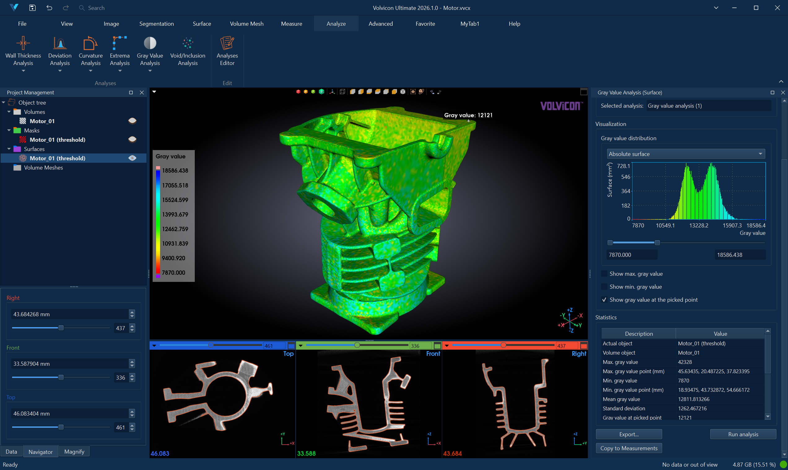
Gray Value Analysis

The Gray Value Analysis tool maps grayscale intensity values from volume image data onto mask or surface geometry, enabling visualization and statistical analysis of material density or intensity distribution across an object's surface. This analysis bridges volumetric image data with geometric representations, supporting applications in material characterization, density mapping, and CT value analysis.

Understanding Gray Value Mapping

Gray value analysis samples the underlying volume image at each point on a mask or surface object and assigns the corresponding intensity value to that location. For medical CT data, these values typically represent Hounsfield units (HU) that correlate with material density. For industrial CT or other imaging modalities, the values reflect the material's X-ray attenuation or other physical properties.

The analysis produces a color-mapped visualization on the object's surface, revealing how material properties vary across the geometry. Statistical summaries provide quantitative metrics for the intensity distribution.

Hounsfield Units in CT

In CT imaging, Hounsfield units (HU) provide a standardized scale where water = 0 HU and air = -1000 HU. Different tissues and materials have characteristic HU ranges:

• Bone: 400 to 1000+ HU
• Soft tissue: 40 to 80 HU
• Fat: -100 to -50 HU
• Air: -1000 HU

Accessing the Tool

1. Navigate to the Analyze ribbon tab.
2. Click the Gray Value Analysis button.
3. Select the analysis mode from the dropdown menu:
   • Analyze Mask – Analyze gray values on a mask object's 3D preview surface.
   • Analyze Surface – Analyze gray values on a triangle mesh surface object.

Analysis Configuration

Creating a New Analysis

1. In the Analysis Selection section, click Select analysis to open the Gray Value Analysis Editor dialog.
2. Click New Analysis to create a new analysis configuration.
3. Configure the analysis parameters (detailed below).
4. Click Load to load the selected analysis and close the dialog.

Analysis Parameters

Parameter	Description
Analysis Name	User-defined name for the analysis. Double-click to rename.
Actual Object	The mask or surface object to analyze.
Volume Object	The volume image from which to sample gray values.
Surface Quality	(Mask analysis only) Quality of the 3D preview surface: Optimal, High, Medium, or Low.
Above Max. Range Color	Color displayed for gray values above the visualization range.
LUT	Lookup table (color map) for visualizing gray values.
Below Min. Range Color	Color displayed for gray values below the visualization range.
Range (GV)	Current visualization range in gray value units (read-only, updated after analysis).

Selecting the Volume Object

The Volume Object parameter specifies which volume image to use for sampling gray values. This is particularly important when:

• Multiple volume images are loaded in the project
• You want to analyze the same geometry against different imaging data
• Comparing original vs. processed volume images

note

The volume object must spatially overlap with the mask or surface being analyzed. If the geometry extends beyond the volume boundaries, those regions will not have valid gray values.

Running the Analysis

1. After loading an analysis configuration, click Run Analysis.
2. A progress dialog appears while the analysis samples gray values.
3. Upon completion:
   • The object displays color-mapped gray values in 3D and 2D views.
   • The histogram updates with the gray value distribution.
   • The statistics table populates with summary metrics.

Interpreting Results

Visualization

The analyzed object displays a color gradient representing gray values sampled from the volume:

• Cool colors (blue): Lower gray values (typically less dense materials)
• Warm colors (red): Higher gray values (typically denser materials)

The color mapping reveals material variations and density gradients across the object's surface.

Statistics

The statistics table displays key metrics:

Statistic	Description
Actual Object	Name of the analyzed object.
Volume Object	Name of the source volume image.
Maximum Gray Value	Highest sampled intensity value.
Maximum Point	Coordinates of the maximum intensity location.
Minimum Gray Value	Lowest sampled intensity value.
Minimum Point	Coordinates of the minimum intensity location.
Mean Gray Value	Average intensity across all sampled points.
Standard Deviation	Variation in gray values.
Range	Current visualization range.
Area Below Min. Range (%)	Percentage of surface below the minimum range.
Area Above Max. Range (%)	Percentage of surface above the maximum range.
Area Within Range (%)	Percentage of surface within the selected range.

Interactive Features

Feature	Description
Show Maximum	Displays an annotation at the point of highest gray value.
Show Minimum	Displays an annotation at the point of lowest gray value.
Pick Point	Enable interactive picking to display gray values at any clicked location.

Typical Workflows

Bone Density Visualization

1. Segment the bone structure to create a mask.
2. Create a Gray Value Analysis with the CT volume as the reference.
3. Run the analysis.
4. Adjust the visualization range to highlight density variations.
5. Identify regions of low bone density (potential osteoporosis).

Material Characterization

1. Import or segment the part to analyze.
2. Configure Gray Value Analysis with the appropriate volume.
3. Run the analysis to map material density.
4. Use the histogram to identify different material phases.
5. Set range thresholds to distinguish between materials.

Porosity Assessment

1. Analyze the surface of a cast or printed part.
2. Look for regions with lower gray values indicating voids or porosity.
3. Use Show Minimum to locate the least dense areas.
4. Compare statistics against reference specifications.

Multi-Volume Comparison

1. Load both original and processed volume images.
2. Create two Gray Value Analyses for the same geometry.
3. Reference different volumes in each analysis.
4. Compare results to assess processing effects.

CT Value Mapping for Implant Planning

1. Segment the anatomical structure.
2. Analyze gray values using the CT volume.
3. Identify bone density distribution for implant placement.
4. Export results for surgical planning documentation.

Histogram Types

The histogram visualization supports three display modes:

Type	Description
Absolute surface	Shows the actual surface area (mm²) for each gray value bin.
Relative surface	Displays surface area as a percentage of total.
Cumulative relative surface	Shows accumulated percentage across gray value bins.

Exporting Results

CSV Export

Click Export and select CSV to save:

• Statistical summary data
• Gray value distribution histogram data
• Per-point gray values (optional)

PDF Report

Click Export and select PDF Report to generate a formatted document containing:

• Analysis configuration and parameters
• 3D visualization screenshots
• Histogram and statistics
• Intensity location annotations

See PDF Report for detailed report customization options.

Best Practices

1. Ensure spatial alignment: The mask or surface must be spatially aligned with the volume data. Use the same coordinate system for accurate sampling.

2. Use appropriate surface quality: Higher quality settings provide more sample points and better representation of gray value variations.

3. Consider interpolation effects: Gray values are interpolated from the volume grid. Very fine surfaces may show interpolation artifacts.

4. Document the volume source: Always record which volume image was used for the analysis, especially when multiple volumes exist.

5. Calibrate expectations: Understand the gray value range and units of your specific imaging modality for meaningful interpretation.

6. Check volume coverage: Ensure the geometry is fully contained within the volume bounds for complete analysis.

Troubleshooting

Issue	Possible Cause	Solution
Gray values appear uniform or incorrect	Wrong volume object selected	Verify the correct volume is specified
Missing values in some regions	Geometry extends beyond volume	Crop geometry to volume bounds or expand volume
Unexpected value range	Different imaging modality or scaling	Check volume properties and adjust range accordingly
Noisy gray value distribution	High-frequency variations in volume	Consider smoothing the volume before analysis

Related Resources

• Analyze Tab Overview – Overview of all analysis tools
• Curvature Analysis – Analyze surface geometry properties
• Volume Statistics – Statistical analysis of volume data
• Histogram – Interactive histogram visualization
• PDF Report – Generate analysis reports
• Analysis Operations API – Scripting support for analysis automation